Principal Component Analysis of AOP Hyperspectral Data in GEE

The principal components (PC) transform is a spectral rotation that takes spectrally correlated image data and outputs uncorrelated data. This can be a useful tool, especially for the high-dimensional AOP data, which is comprised of 426 bands (~380 valid bands, excluding the water vapor and noisy bands). Many of these bands may be correlated, so PCA can be a useful first step for reducing dimensionality and creating a more manageable (smaller) dataset to work with for further analysis, without reducing the essential information.

For this example, we'll use bidirectional reflectance data over the NEON site Little Rock Lake (LIRO) in Wisconsin.

Script 1: Computing PCA

Read in the AOP Directional Reflectance Image

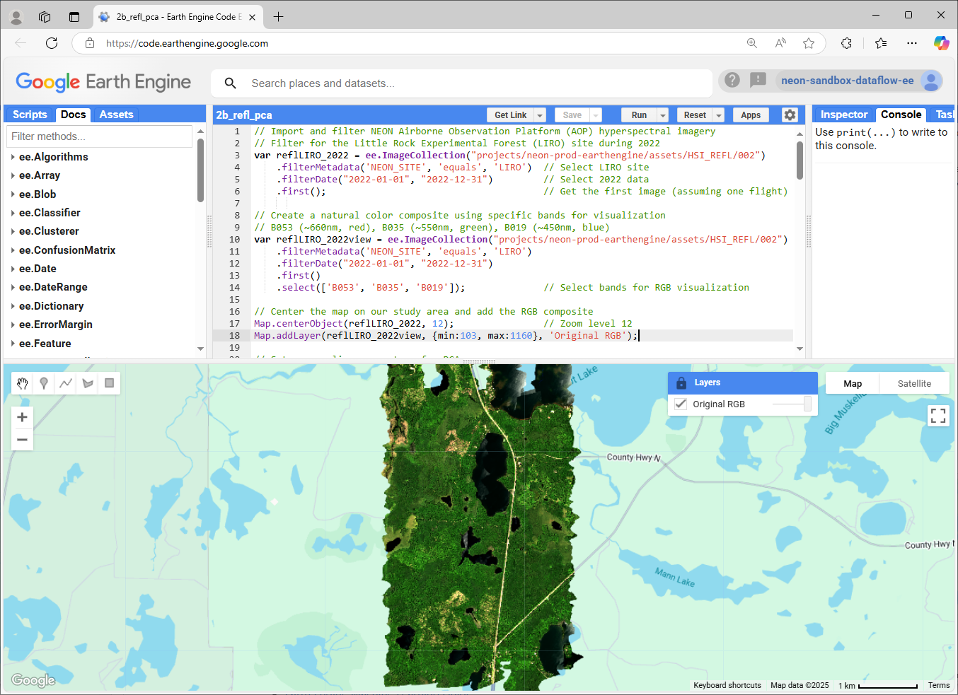
First, we'll import the hyperspectral data and create a natural color composite for visualization:

// Import and filter NEON AOP hyperspectral imagery
var reflLIRO_2022 = ee.ImageCollection("projects/neon-prod-earthengine/assets/HSI_REFL/002")
  .filterMetadata('NEON_SITE', 'equals', 'LIRO') // Select LIRO site
  .filterDate("2022-01-01", "2022-12-31") // Select 2022 data
  .first(); // Get the first image

// Create RGB visualization using specific bands
var reflLIRO_2022view = ee.ImageCollection("projects/neon-prod-earthengine/assets/HSI_REFL/002")
  .filterMetadata('NEON_SITE', 'equals', 'LIRO')
  .filterDate("2022-01-01", "2022-12-31")
  .first().select(['B053', 'B035', 'B019']); // Select bands for RGB visualization

// Center on the LIRO reflectance dataset
Map.centerObject(reflLIRO_2022, 12);

// Add the layer to the Map
Map.addLayer(reflLIRO_2022view, {min:103, max:1160}, 'Original RGB');

Set up Sampling for PCA

You can run PCA on an entire image, but this would be very memory intensive. Instead, we can use representative samples to compute the covariance matrix, which will provide similar results but run much more quickly. For this example, we'll collect 500 random samples. On your own you can try out different sample sizes to get a better understanding of the trade-offs.

var numberOfSamples = 500;

var sample = reflLIRO_2022.sample({
  region: reflLIRO_2022.geometry(),
  scale: 10,
  numPixels: numberOfSamples,
  seed: 1,
  geometries: true
});

var samplePoints = ee.FeatureCollection(sample);

Create Helper Functions

We need two main helper functions to generate the PCA. The first function generates band names and the second calculates the PCA.

// Function to generate names for the principal component bands
// Example: PC1, PC2, PC3, etc.
function getNewBandNames(prefix, num) {
    return ee.List.sequence(1, num).map(function(i) {
        return ee.String(prefix).cat(ee.Number(i).int().format());
    });
}

/// Function to perform Principal Component Analysis
function calcImagePca(image, numComponents, samplePoints) {
    // Convert the image into an array for matrix operations
    var arrayImage = image.toArray();
    var region = samplePoints.geometry();
    
    // Calculate mean values for each band
    var meanDict = image.reduceRegion({
        reducer: ee.Reducer.mean(),
        geometry: region,
        scale: 10,
        maxPixels: 1e13,
        bestEffort: true,
        tileScale: 16                               // Parameter to prevent computation timeout
    });
    
    // Center the data by subtracting the mean
    var meanImage = ee.Image.constant(meanDict.values(image.bandNames()));
    var meanArray = meanImage.toArray().arrayRepeat(0, 1);
    var meanCentered = arrayImage.subtract(meanArray);
    
    // Calculate the covariance matrix
    var covar = meanCentered.reduceRegion({
        reducer: ee.Reducer.centeredCovariance(),
        geometry: region,
        scale: 10,
        maxPixels: 1e13,
        bestEffort: true,
        tileScale: 16
    });
    
    // Compute eigenvalues and eigenvectors
    var covarArray = ee.Array(covar.get('array'));
    var eigens = covarArray.eigen();
    var eigenVectors = eigens.slice(1, 1);  // Extract eigenvectors
    
    // Project the mean-centered data onto the eigenvectors
    var principalComponents = ee.Image(eigenVectors)
        .matrixMultiply(meanCentered.toArray(1));
    
    // Return the desired number of components
    return principalComponents
        .arrayProject([0])  // Project the array to 2D
        .arraySlice(0, 0, numComponents); // Select the first n components
}

Apply PCA and Export Results

Now we'll apply the PCA to the LIRO hyperspectral image and export the results. Change the assetId tag below to point to your cloud project. This exporting step can take several minutes to complete, and longer if you are using a larger AOP image.

// Apply PCA to the hyperspectral image
var numComponents = 5;                              // Number of components to retain
var pcaImage = calcImagePca(reflLIRO_2022, numComponents, samplePoints);
var bandNames = getNewBandNames('PC', numComponents);
var finalPcaImage = pcaImage.arrayFlatten([bandNames]);  // Convert to regular image

// Export the PCA results to Earth Engine Assets, changing the assetId so that it points to your cloud project
// This step may take around 10 minutes to complete
Export.image.toAsset({
    image: finalPcaImage,
    description: 'PCA_LIRO_2022',
    assetId: 'projects/neon-sandbox-dataflow-ee/assets/PCA_LIRO_2022', // change this to your cloud project
    scale: 1,                                       // Output resolution in meters
    maxPixels: 1e13                                 // Increase max pixels for large exports
});

Script 2: Visualizing PCA Results and K-Means Classification

Now that we've exported the 5 principal components, let's try to understand the results. We will then apply a K-means clustering algorithm to carry out a basic classification, to show that we can run a similar analysis on the dimensionally-reduced dataset.

Part 1: Visualizing PCA Results

After the export completes, run this second script to visualize the Principal Components:

// Load the original hyperspectral image, selecting bands for RGB visualization
// B053 (~660nm, red), B035 (~550nm, green), B019 (~450nm, blue)
var reflLIRO_2022view = ee.ImageCollection("projects/neon-prod-earthengine/assets/HSI_REFL/002")
    .filterMetadata('NEON_SITE', 'equals', 'LIRO')  // Select LIRO experimental forest site
    .filterDate("2022-01-01", "2022-12-31")         // Select 2022 data
    .first()                                        // Get first (and likely only) image
    .select(['B053', 'B035', 'B019']);              // Select bands for natural color display

// Load the pre-computed PCA results from Earth Engine Assets
// This asset was created by Script 1 and contains the first 5 principal components
var pcaAsset = ee.Image('projects/neon-sandbox-dataflow-ee/assets/PCA_LIRO_2022');

print("PCA image - top 5 PCA bands", pcaAsset)

// Center the map on our study area
// Zoom level 12 provides a good overview of the LIRO site
Map.centerObject(reflLIRO_2022view, 13);

// Add layers to the map
// Start with the original RGB image as the base layer
Map.addLayer(reflLIRO_2022view, 
    {min: 103, max: 1160},                          // Set visualization parameters
    'Original RGB');                                 // Layer name in the Layer Manager

// Pull in the palettes package and create a spectral color palette for visualization
var palettes = require('users/gena/packages:palettes');
var pc1_palette = palettes.colorbrewer.Spectral[9]

// Add the first and second principal components as layers
// PC1 typically contains the most variance/information from the original bands
Map.addLayer(pcaAsset,
    {bands: ['PC1'],                                // Display the first component
     min: -7000, max: 40000,                        // Set stretch values for good contrast
    palette: pc1_palette,},                         // Add a the pc1_palette
    'PC1');                                         // Layer name

Map.addLayer(pcaAsset,
    {bands: ['PC2'],                                // Display the second component
     min: -7000, max: 40000,                        // Set stretch values for good contrast
    palette: pc1_palette,},                         // Add a the pc1_palette
    'PC1');                                         // Layer name

// Note: You can toggle layer visibility and adjust transparency
// using the Layer Manager panel in the upper right of the map

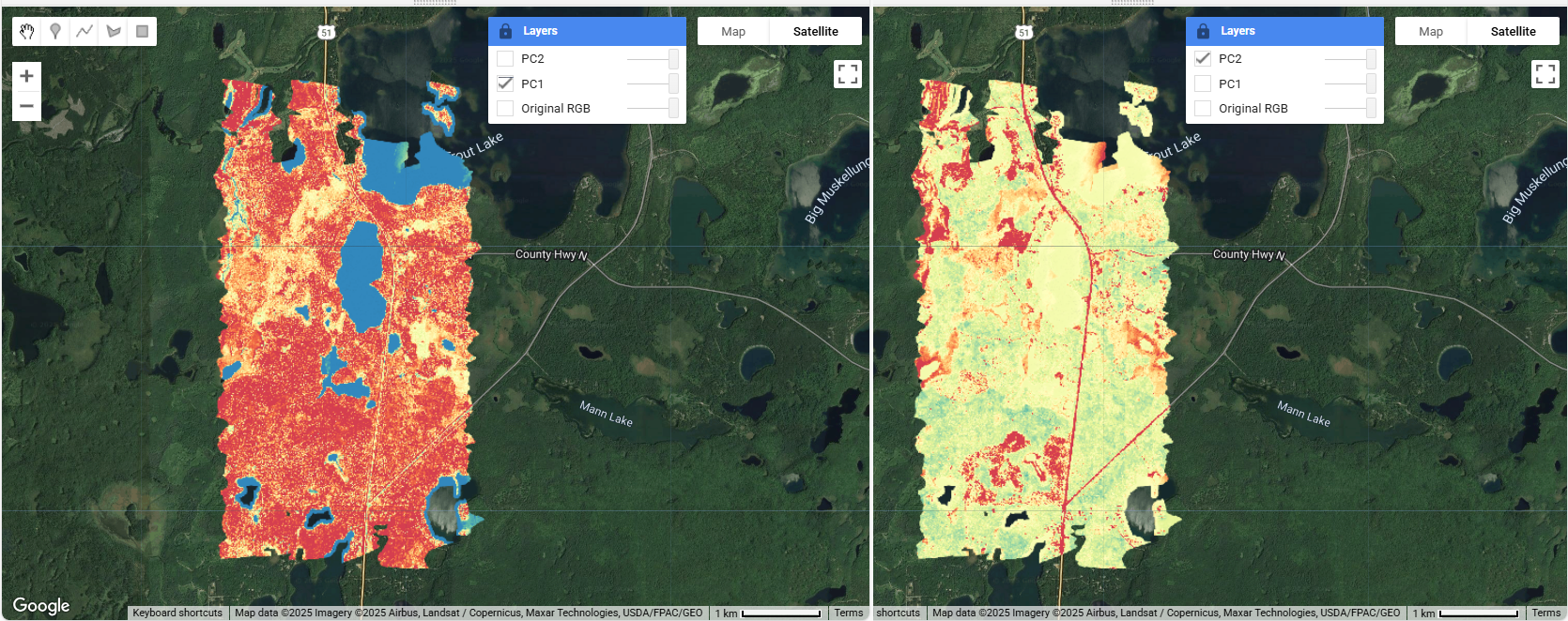
Interpreting Principal Components

• PC1: Usually represents overall brightness/albedo variations (typically 90%+ of variance)
• PC2: Often highlights vegetation vs. non-vegetation contrasts
• PC3: May reveal subtle features not visible in original bands

On your own:

1. Compare PC1 with the original RGB image to understand major landscape features
2. Add PC3 to the map as a layer, and look for patterns in PC2 and PC3 that might reveal hidden information
3. Consider how different PCs might be useful for your specific research questions

Part 2: K-Means Classification

Now that we've run the PCA, we can use the condensed 5-band version of the data instead of the full hyperspectral dataset for further analysis. In this example, we'll show how to run a k-means clustering analysis. Kmeans is a popular unsupervized clustering algorithm for carrying out classification when you don't have training data. The code below shows how to do this:

// Create training dataset from PCA results
var training = pcaAsset.sample({
    region: pcaAsset.geometry(),
    scale: 10,
    numPixels: 5000,
    seed: 123
});

// Function to perform clustering with different numbers of clusters
function performClustering(numClusters) {
    // Train the clusterer
    var clusterer = ee.Clusterer.wekaKMeans({
        nClusters: numClusters,
        seed: 123
    }).train(training);
    
    // Cluster the PCA image
    var clustered = pcaAsset.cluster(clusterer);
    
    // Add clustered image to map
    Map.addLayer(clustered.randomVisualizer(), {}, 
        'Clusters (k=' + numClusters + ')');
    
    return clustered;
}

// Try different numbers of clusters
var clusters5 = performClustering(5);
var clusters7 = performClustering(7);
var clusters10 = performClustering(10);

// Optional: Calculate and export cluster statistics
var calculateClusterStats = function(clusteredImage, numClusters) {
    // Calculate area per cluster
    var areaImage = ee.Image.pixelArea().addBands(clusteredImage);
    var areas = areaImage.reduceRegion({
        reducer: ee.Reducer.sum().group({
            groupField: 1,
            groupName: 'cluster',
        }),
        geometry: pcaAsset.geometry(),
        scale: 10,
        maxPixels: 1e13
    });
    
    print('Cluster areas (m²) for k=' + numClusters, areas);
};

calculateClusterStats(clusters5, 5);
calculateClusterStats(clusters7, 7);
calculateClusterStats(clusters10, 10);

// Uncomment to export clustered results to your Google Drive, if desired
// Export.image.toDrive({
//     image: clusters5,
//     description: 'LIRO_PCA_Clusters_k5',
//     scale: 5,
//     maxPixels: 1e13
// });

Recap

In this lesson you:

• Created a workflow that handles large datasets efficiently
• Learned how to implement Pricipal Component Analysis (PCA) on hyperspectral data in GEE
• Visualized and exported transformed data
• Gained experience interpreting PCA results
• Gained experience running k-Means clustering and interpreting results

Acknowledgment and References

Thanks to Kel Markert (Google Cloud Geographer), for his help in developing the representative sampling code as a memory-efficient option to compute PCA.

This tutorial was made with help from AI, which pulled from the following sources:

Cawse-Nicholson, K., Townsend, P.A., Schimel, D. et al. (2021). NASA's surface biology and geology designated observable: A perspective on surface imaging algorithms. Remote Sensing of Environment, 257, 112349.

• Paper discussing hyperspectral imaging algorithms including preprocessing workflows

Datt, B., McVicar, T. R., Van Niel, T. G., Jupp, D. L., & Pearlman, J. S. (2003). Preprocessing EO-1 Hyperion hyperspectral data to support the application of agricultural indexes. IEEE Transactions on Geoscience and Remote Sensing, 41(6), 1246-1259.

• Discusses preprocessing steps for hyperspectral data

Deschamps, B., McNairn, H., Shang, J., & Jiao, X. (2012). Towards operational radar-only crop type classification: comparison of a traditional decision tree with a random forest classifier. Canadian Journal of Remote Sensing, 38(1), 60-68.

• Application of PCA and clustering for classification

Green, A. A., Berman, M., Switzer, P., & Craig, M. D. (1988). A transformation for ordering multispectral data in terms of image quality with implications for noise removal. IEEE Transactions on Geoscience and Remote Sensing, 26(1), 65-74.

• Classic paper introducing PCA for dimensionality reduction in remote sensing

National Ecological Observatory Network. (2023). Data Tutorial: Introduction to Hyperspectral Remote Sensing Data. https://www.neonscience.org/resources/learning-hub/tutorials/hsi-hdf5-r

• NEON's introduction to hyperspectral data

Plaza, A., Benediktsson, J. A., Boardman, J. W., Brazile, J., Bruzzone, L., Camps-Valls, G., ... & Trianni, G. (2009). Recent advances in techniques for hyperspectral image processing. Remote Sensing of Environment, 113, S110-S122.

• Comprehensive review of hyperspectral processing techniques including PCA

Wang, J., & Chang, C. I. (2006). Independent component analysis-based dimensionality reduction with applications in hyperspectral image analysis. IEEE Transactions on Geoscience and Remote Sensing, 44(6), 1586-1600.

• Comparison of PCA with other dimensionality reduction techniques

Get Lesson Code

Reflectance PCA Analysis & KMeans Classification: Part 1

Reflectance PCA Analysis & KMeans Classification: Part 2