Wildfire Change Exploration Using AOP Reflectance and Canopy Height Data in GEE

GEE is a great place to conduct exploratory analysis to better understand the datasets you are working with. In this lesson, we will show how to pull in AOP Surface Directional Reflectance (SDR) data, as well as the Ecosystem Structure (Canopy Height Model - CHM) data to look at interannual differences at the NEON site Great Smokey Mountains (GRSM), where the Chimney Tops 2 Fire broke out in late November 2016. NEON data over the GRSM site collected in June 2016 and October 2017 captures most of the burned area and presents a unique opportunity to study wildfire effects on the ecosystem and analysis of post-wildfire vegetation recovery. In this lesson, we will calculate the differenced Normalized Burn Ratio (dNBR) between 2017 and 2016, and also create a CHM difference raster to highlight vegetation structure differences in the burned area. We will also pull in Landsat satellite data and create a time-series of the NBR within the burn perimeter to look at annual differences.

Using remote sensing data to better understand wildfire impacts is an active area of research. In April 2023, Park and Sim published an Open Access paper titled "Characterizing spatial burn severity patterns of 2016 Chimney Tops 2 fire using multi-temporal Landsat and NEON LiDAR data". We encourage you to read this paper for an example of wildfire research using AOP remote sensing and satellite data. This lesson provides an introduction to conducting this sort of analysis in Google Earth Engine.

Functions to Read in SDR and CHM Image Collections

Let's get started. The code in the beginning of this lesson should look familiar from the previous tutorials in this series. In this first chunk of code, we will the center location of GRSM, and read in the fire perimeter as a FeatureCollection.

// Specify center location and flight box for GRSM (https://www.neonscience.org/field-sites/grsm)
var site_center = ee.Geometry.Point([-83.5, 35.7])

// Read in the Chimney Tops fire perimeter shapefile
var ct_fire_boundary = ee.FeatureCollection('projects/neon-sandbox-dataflow-ee/assets/chimney_tops_fire')

Next, we'll read in the SDR image collection, and then write a function to mask out the cloudy weather data, and use the map feature to apply this to our SDR collection at GRSM.

// Read in the SDR Image Collection at GRSM
var grsm_sdr_col = ee.ImageCollection('projects/neon-prod-earthengine/assets/HSI_REFL/001')
  .filterBounds(site_center)
  
// Function to mask out poor-weather data, keeping only the <10% cloud cover weather data
function clearSDR(image) { 
  // create a single band Weather Quality QA layer 
  var weather_qa = image.select(['Weather_Quality_Indicator']);
  // WEATHER QUALITY INDICATOR = 1 is < 10% CLOUD COVER
  var clear_qa = weather_qa.eq(1);
  // mask out all cloudy pixels from the SDR image
  return image.updateMask(clear_qa);
}

// Use map to apply the clearSDR function to the SDR collection and return a clear-weather subset of the data
var grsm_sdr_cloudfree = grsm_sdr_col.map(clearSDR)

Next let's write a function to display the NIS images from 2016, 2017, and 2021 in GEE. For more details on how this function works, you can refer to the tutorial Functions in Google Earth Engine (GEE).

// Function to display individual (yearly) SDR Images
function addSDRImage(image) { 
  var image_id = ee.Image(image.id); // get the system:id and convert to string
  var sys_id = ee.String(image_id.get("system:id")).getInfo();  // get the system:id - this is an object on the server
  var filename = sys_id.slice(52,100); // extract the fileName (NEON domain + site code + product code + year)
  var image_rgb = image_id.select(['B053', 'B035', 'B019']);  // select only RGB bands for display
  
  Map.addLayer(image_rgb, {min:220, max:1600}, filename, 1)   // add RGB composite to the map
}

// call the addNISimages function to add SDR layers to map
grsm_sdr_col.evaluate(function(grsm_sdr_col) {
  grsm_sdr_col.features.map(addSDRImage);
})

Next we can create a similar function for reading in the CHM dataset over all the years. The main differences between this function and the previous one are that 1) it is set to display a single band image, and 2) instead of hard-coding in the minimum and maximum values to display, we dynamically determine them from the data itself, so it will scale appropriately.

// Read in the CHM Image collection at GRSM
var grsm_chm_col =  ee.ImageCollection('projects/neon-prod-earthengine/assets/CHM/001')
  .filterBounds(site_center)

// Function to display Single Band Images setting display range to linear 2%
function addSingleBandImage(image) { // display each image in collection
  var image_id = ee.Image(image.id); // get the system:id and convert to string
  var sys_id = ee.String(image_id.get("system:id")).getInfo(); 
  var filename = sys_id.slice(52,100); // extract the fileName (NEON domain + site code + product code + year)

  // Dynamically determine the range of data to display
  // Sets color scale to show all but lowest/highest 2% of data
  var pct_clip = image_id.reduceRegion({
    reducer: ee.Reducer.percentile([2, 98]),
    scale: 10,
    maxPixels: 3e7});

  var keys = pct_clip.keys();
  var pct02 = ee.Number(pct_clip.get(keys.get(0))).round().getInfo()
  var pct98 = ee.Number(pct_clip.get(keys.get(1))).round().getInfo()
    
  Map.addLayer(image_id, {min:pct02, max:pct98, palette: chm_palette}, filename, 0)
}

// Call the addSingleBandImage function to add CHM layers to map 
grsm_chm_col.evaluate(function(grsm_chm_col) {
  grsm_chm_col.features.map(addSingleBandImage);
})

// Center the map on GRSM and set zoom level to 12
Map.setCenter(-83.5, 35.6, 12);

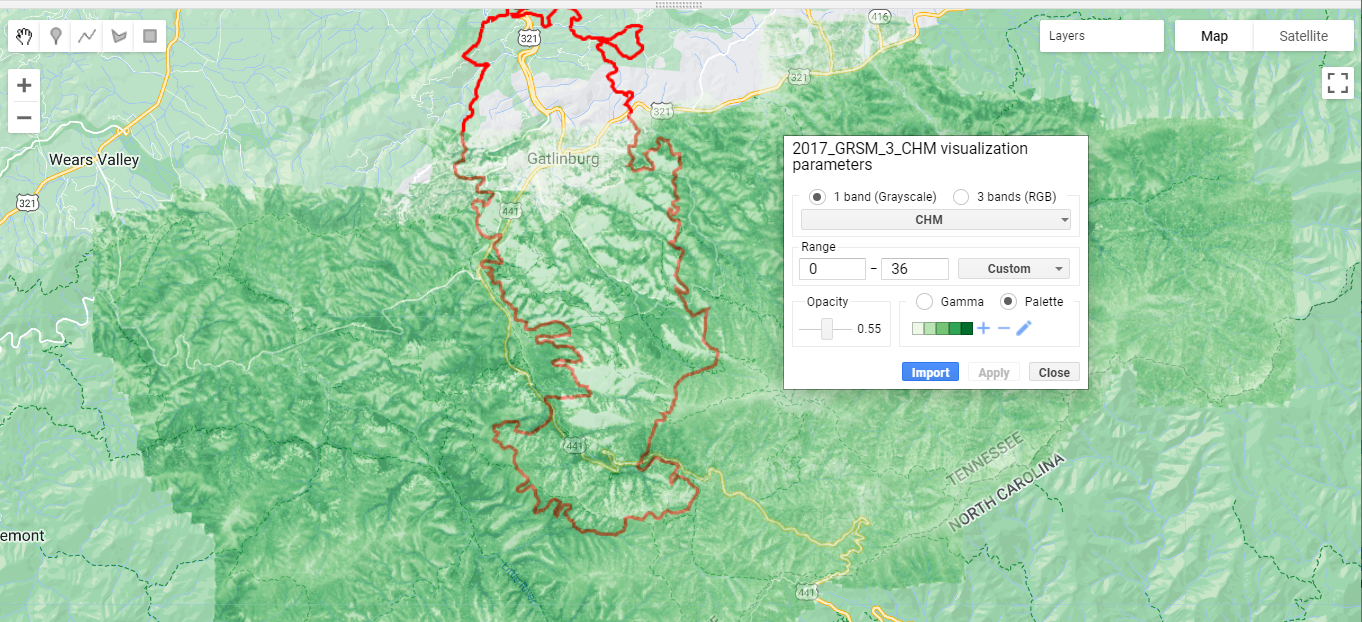
Now that you've read in these two datasets (SDR and CHM) over all the years of available data, we encourage you to explore the different layers and see what you notice! Toggle between the layers, play with the opacity. Visual inspection is an important first step in exploratory analysis - see if you can recognize patterns and form new questions based off what you see.

CHM Difference Layers

Next let's create a new raster layer of the difference between the CHMs from 2 different years.

// Difference the CHMs from 2017 and 2016 and 2021
var grsm_chm2021 = grsm_chm_col.filterDate('2021-01-01', '2021-12-31').first();
var grsm_chm2017 = grsm_chm_col.filterDate('2017-01-01', '2017-12-31').first();
var grsm_chm2016 = grsm_chm_col.filterDate('2016-01-01', '2016-12-31').first();

// Subtract the CHMs to create difference CHM rasters
var chm_diff_2017_2016 = grsm_chm2017.subtract(grsm_chm2016);
var chm_diff_2021_2017 = grsm_chm2021.subtract(grsm_chm2017);
var chm_diff_2021_2016 = grsm_chm2021.subtract(grsm_chm2016);

// Display the first CHM difference raster (2017-2016) and add as a layer to the Map
print('CHM Difference 2017-2016',chm_diff_2017_2016)

Map.addLayer(chm_diff_2017_2016, {min: -10, max: 10, palette: dchm_palette}, 'CHM diff 2017-2016');

CHM Difference Stats and Histograms

Next let's calculate the mean difference in Canopy Height inside the fire perimeter for the various years. We'll also plot histograms of the CHM differences.

// Calculate the mean dCHM between the various years:
print('Mean dCHM in the Chimney Tops Fire Perimeter')

print('Mean dCHM 2017-2016',chm_diff_2017_2016.reduceRegion({
      reducer: ee.Reducer.mean(),
      geometry: ct_fire_boundary,
      scale: 30}));
      
print('Mean dCHM 2021-2017',chm_diff_2021_2017.reduceRegion({
      reducer: ee.Reducer.mean(),
      geometry: ct_fire_boundary,
      scale: 30}));
      
print('Mean dCHM 2021-2016',chm_diff_2021_2016.reduceRegion({
      reducer: ee.Reducer.mean(),
      geometry: ct_fire_boundary,
      scale: 30}));

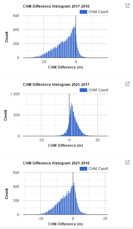
In the console, if you expand the objects, you can see that from 2016-2017, there was a net loss in canopy height of ~6.6m, and between 2017-2021 there was a net growth of ~3m, suggesting a considerable amount of re-growth in the 5 years after the fire.

We can also look at the histograms of the CHM differences to provide a little more information about the ecosystem structure dynamics immediately after the fire and in the subsequent years. To plot histograms, first write a function to create a histogram given a difference CHM raster (calculated above) and a string of the years that are being differenced, as inputs. The string is just used to include in the histogram chart title.

// Function to create histogram charts for each CHM difference layer, clipped by the chimney tops fire perimeter
function chmDiffHist(img,years_str) { 
  var hist =
      ui.Chart.image.histogram({image: img.clip(ct_fire_boundary), region: ct_fire_boundary, scale: 50})
          .setOptions({title: 'CHM Difference Histogram ' + years_str,
                      hAxis: {title: 'CHM Difference (m)',titleTextStyle: {italic: false, bold: true},},
                      vAxis: {title: 'Count', titleTextStyle: {italic: false, bold: true}},});
  return hist
}

// Apply the function to the three CHM difference rasters
var chm_diff_hist_2017_2016 = chmDiffHist(chm_diff_2017_2016,'2017-2016')
var chm_diff_hist_2021_2016 = chmDiffHist(chm_diff_2021_2016,'2021-2016')
var chm_diff_hist_2021_2017 = chmDiffHist(chm_diff_2021_2017,'2021-2017')

// Display the CHM difference histograms charts on the Console
print(chm_diff_hist_2017_2016);
print(chm_diff_hist_2021_2017);
print(chm_diff_hist_2021_2016);

On your own, try to interpret what these difference histograms are showing.

Normalized Burn Ratio (NBR)

Last but not least, we can take a quick look at the NBR and dNBR. Refer to the CU Earth Lab dNBR Lesson for a nice explanation of this metric in the context of multispectral satellite data.

// Read in clear SDR images at GRSM in 2016, 2017, and 2021 
var grsm_sdr2016_clear = grsm_sdr_cloudfree.filterDate('2016-01-01', '2016-12-31').first()
var grsm_sdr2017_clear = grsm_sdr_cloudfree.filterDate('2017-01-01', '2017-12-31').first();
var grsm_sdr2021_clear = grsm_sdr_cloudfree.filterDate('2021-01-01', '2021-12-31').first();
  
//------------------------- Normalized Difference Burn Ratio ----------------------------
// The normalized burn ratio (NBR) is a normalized difference index using the shortwave-infrared (SWIR) and near-infrared (NIR) portions of the electromagnetic spectrum. dNBR can be used as a metric to map fire extent and burn severity when calculating the difference between pre and post fire conditions.

// calculate NBR for the 3 years
// B097: B365: 
var sdr_pre_nbr_2016 = grsm_sdr2016_clear.normalizedDifference(['B097', 'B365']);
var sdr_post_nbr_2017 = grsm_sdr2017_clear.normalizedDifference(['B097', 'B365']);
var sdr_post_nbr_2021 = grsm_sdr2021_clear.normalizedDifference(['B097', 'B365']);

// calculate dNBR 2016-2017 and 2016-2021
var sdr_dNBR_2016_2017 = sdr_pre_nbr_2016
                            .subtract(sdr_post_nbr_2017)
                            .clip(ct_fire_boundary);

var sdr_dNBR_2016_2021 = sdr_pre_nbr_2016
                            .subtract(sdr_post_nbr_2021)
                            .clip(ct_fire_boundary);

// Remove comment-symbols (//) below to display pre- and post-fire NBR as layers
// Map.addLayer(sdr_pre_nbr_2016, {min: -1, max: 1, palette: red_ylw_grn}, 'Pre-fire (June 2016) Normalized Burn Ratio');
// Map.addLayer(sdr_post_nbr_2017, {min: -1, max: 1, palette: red_ylw_grn}, 'Post-fire (Oct 2017) Normalized Burn Ratio');
// Map.addLayer(sdr_post_nbr_2021, {min: -1, max: 1, palette: red_ylw_grn}, 'Post-fire (June 2021) Normalized Burn Ratio');

// add dNBR layers
Map.addLayer(sdr_dNBR_2016_2017, {min: -1, max: 1, palette: dnbr_palette}, 'dNBR 2016-2017');
Map.addLayer(sdr_dNBR_2016_2021, {min: -1, max: 1, palette: dnbr_palette}, 'dNBR 2016-2021');

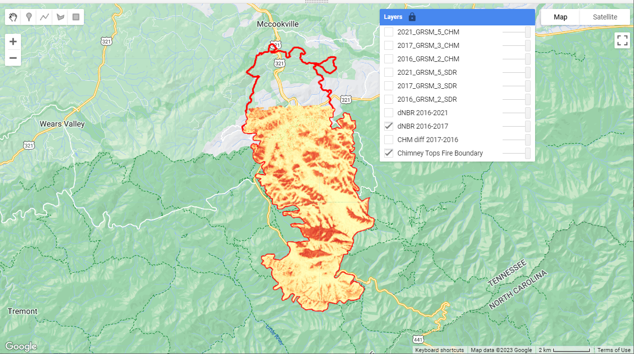
The differenced Normalized Burn Ratio (dNBR) does a great job of highlighting the burned areas (in red).

On your own, we encourage you to dig into the code from this tutorial and expand upon it according to your scientific interests. Think of some questions you have about this dataset and think about how you might answer it using GEE. Modify these functions or try writing your own function to answer your question(s). For example, try out different reducers to compile other statistis to summarize the CHM and NBR differences, or see if there are any other datasets that you could bring in to expand your analysis. This is just the starting point!

Get Lesson Code

GRSM Wildfire Change Exploration