Explore biodiversity with NEON algae data

Introduction

In this code-along tutorial, we will explore how to find and download NEON biodiversity data using the ecocomDP package for R, which has been developed by the Environmental Data Initiative (EDI) in collaboration with NEON staff.

What is ecocomDP?

"ecocomDP" is both the name of an R package and a data model.

EDI describes the ecocomDP data model as "A dataset design pattern for ecological community data to facilitate synthesis and reuse".

See the ecocomDP github repo here: https://github.com/EDIorg/ecocomDP.

The motivation is for both NEON biodiversity data products and EDI data packages, including data from the US Long Term Ecological Research Network and Macrosystems Biology projects, to be discoverable through a single data search tool, and to be delivered in a standard format. Our objective here is to demonstrate how the workflow will work with NEON biodiversity data packages.

Load Libraries and Prepare Workspace

First, we will load all necessary libraries into our R environment. If you have not already installed these libraries, please see the 'R Packages to Install' section above.

There are also two optional sections in this code chunk: clearing your environment, and loading your NEON API token. Clearing out your environment will erase all of the variables and data that are currently loaded in your R session. This is a good practice for many reasons, but only do this if you are completely sure that you won't be losing any important information! Secondly, your NEON API token will allow you increased download speeds, and helps NEON anonymously track data usage statistics, which helps us optimize our data delivery platforms, and informs our monthly and annual reporting to our funding agency, the National Science Foundation. Please consider signing up for a NEON data user account, and using your token as described in this tutorial here.

# clean out workspace

#rm(list = ls()) # OPTIONAL - clear out your environment
#gc()            # Uncomment these lines if desired

# load packages
library(tidyverse)
library(neonUtilities)
library(vegan)
library(ecocomDP)

# source .r file with my NEON_TOKEN
# source("my_neon_token.R") # OPTIONAL - load NEON token
# See: https://www.neonscience.org/neon-api-tokens-tutorial

Download Macroinvertibrate Data

In this first step, we show how to search the ecocomDP database for macroinvertebrate data including those from LTER and NEON sites (and others).

# search for invertebrate data products
my_search_result <- 
    ecocomDP::search_data(text = "invertebrate")
View(my_search_result)

# pull data for the NEON aquatic "Macroinvertebrate
# collection"
my_data <- ecocomDP::read_data(
  id = "neon.ecocomdp.20120.001.001",
  site = "ARIK",
  startdate = "2017-06",
  enddate = "2020-03",
  # token = NEON_TOKEN, #Uncomment to use your token
  check.size = FALSE)

Now that we have downloaded the data, let's take a look at the ecocomDP data object structure:

# examine the structure of the data object that is returned
my_data %>% names()

## [1] "id"                "metadata"          "tables"            "validation_issues"

my_data$id

## [1] "neon.ecocomdp.20120.001.001"

# short list of package summary data
my_data$metadata$data_package_info

## $data_package_id
## [1] "neon.ecocomdp.20120.001.001.20220505163555"
## 
## $taxonomic_group
## [1] "MACROINVERTEBRATES"
## 
## $orig_NEON_data_product_id
## [1] "DP1.20120.001"
## 
## $NEON_to_ecocomDP_mapping_method
## [1] "neon.ecocomdp.20120.001.001"
## 
## $data_access_method
## [1] "original NEON data accessed using neonUtilities v2.1.4"
## 
## $data_access_date_time
## [1] "2022-05-05 16:35:55 MDT"

# validation issues? None if returns an empty list
my_data$validation_issues

## list()

# examine the tables
my_data$tables %>% names()

## [1] "location"              "location_ancillary"    "taxon"                 "observation"           "observation_ancillary"
## [6] "dataset_summary"

my_data$tables$taxon %>% head()

##   taxon_id taxon_rank       taxon_name                                         authority_system authority_taxon_id
## 1    ABLSP      genus  Ablabesmyia sp.                               Roback 1985 and Epler 2001               <NA>
## 2   ACASP1   subclass        Acari sp.                                    Thorp and Covich 2001               <NA>
## 3   ACTSP5      genus Actinobdella sp.             Thorp and Covich 2001; Thorp and Rogers 2016               <NA>
## 4    AESSP     family    Aeshnidae sp.                           Needham, Westfall and May 2000               <NA>
## 5   AGASP1  subfamily     Agabinae sp.                        Larson, Alarie, and Roughley 2001               <NA>
## 6   ANISP1   suborder   Anisoptera sp. Needham, Westfall and May 2000; Merritt and Cummins 2008               <NA>

my_data$tables$observation %>% head()

##   observation_id             event_id                                 package_id    location_id            datetime taxon_id
## 1          obs_1 ARIK.20170712.CORE.1 neon.ecocomdp.20120.001.001.20220505163555 ARIK.AOS.reach 2017-07-12 17:27:00   CAESP5
## 2          obs_2 ARIK.20170712.CORE.1 neon.ecocomdp.20120.001.001.20220505163555 ARIK.AOS.reach 2017-07-12 17:27:00  CERSP10
## 3          obs_3 ARIK.20170712.CORE.1 neon.ecocomdp.20120.001.001.20220505163555 ARIK.AOS.reach 2017-07-12 17:27:00   CLASP5
## 4          obs_4 ARIK.20170712.CORE.1 neon.ecocomdp.20120.001.001.20220505163555 ARIK.AOS.reach 2017-07-12 17:27:00   CLISP3
## 5          obs_5 ARIK.20170712.CORE.1 neon.ecocomdp.20120.001.001.20220505163555 ARIK.AOS.reach 2017-07-12 17:27:00   CORSP4
## 6          obs_6 ARIK.20170712.CORE.1 neon.ecocomdp.20120.001.001.20220505163555 ARIK.AOS.reach 2017-07-12 17:27:00   CRYSP2
##   variable_name     value                   unit
## 1       density 1000.0000 count per square meter
## 2       density  333.3333 count per square meter
## 3       density  333.3333 count per square meter
## 4       density  333.3333 count per square meter
## 5       density  166.6667 count per square meter
## 6       density  833.3333 count per square meter

Basic Data Visualization

The ecocomDP package offers some useful data visualization tools.

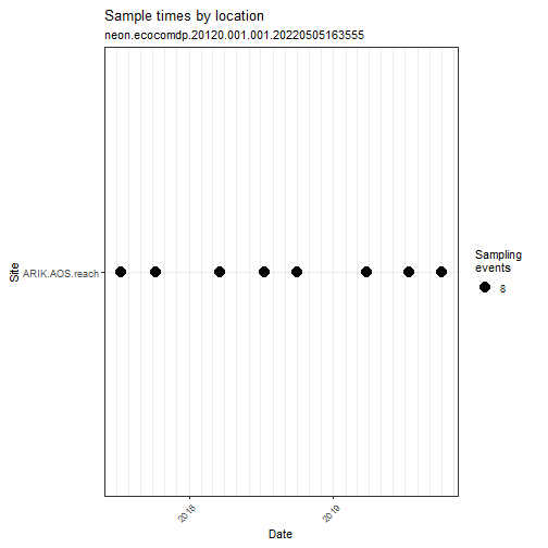
# Explore the spatial and temporal coverage 
# of the dataset
my_data %>% ecocomDP::plot_sample_space_time()

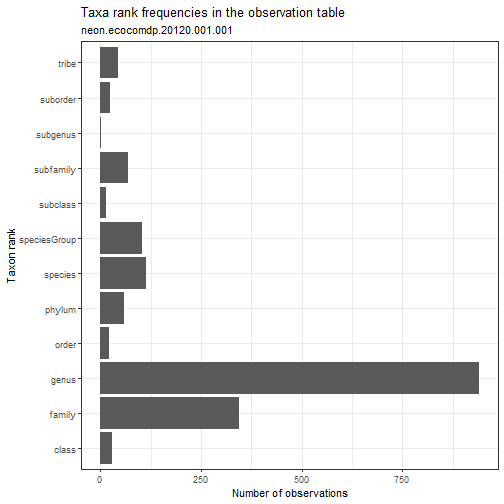
# Explore the taxonomic resolution in the dataset. 
# What is the most common taxonomic resolution (rank) 
# for macroinvertebrate identifications in this dataset?
my_data %>% ecocomDP::plot_taxa_rank()

Search ecocomDP

We can even search for terms in the ecocomDP database using regular expressions:

# search for data sets with periphyton or algae
# regex works!
my_search_result <- ecocomDP::search_data(text = "periphyt|algae")
View(my_search_result)

Let's download the data for the NEON "Periphyton, seston, and phytoplankton collection" from "ARIK" and view its structure:

# pull data for the NEON "Periphyton, seston, and phytoplankton collection" 
# data product
my_data <- 
    ecocomDP::read_data(
      id = "neon.ecocomdp.20166.001.001", 
      site = "ARIK",
      startdate = "2017-06",
      enddate = "2020-03",
      # token = NEON_TOKEN, #Uncomment to use your token
      check.size = FALSE)


# Explore the structure of the returned data object
my_data %>% names()

## [1] "id"                "metadata"          "tables"            "validation_issues"

my_data$metadata$data_package_info

## $data_package_id
## [1] "neon.ecocomdp.20166.001.001.20220505163605"
## 
## $taxonomic_group
## [1] "ALGAE"
## 
## $orig_NEON_data_product_id
## [1] "DP1.20166.001"
## 
## $NEON_to_ecocomDP_mapping_method
## [1] "neon.ecocomdp.20166.001.001"
## 
## $data_access_method
## [1] "original NEON data accessed using neonUtilities v2.1.4"
## 
## $data_access_date_time
## [1] "2022-05-05 16:36:06 MDT"

my_data$validation_issues

## list()

my_data$tables %>% names()

## [1] "location"              "location_ancillary"    "taxon"                 "observation"           "observation_ancillary"
## [6] "dataset_summary"

my_data$tables$location

##      location_id  location_name parent_location_id latitude longitude elevation
## 1            D10 Central Plains               <NA>       NA        NA        NA
## 2           ARIK Arikaree River                D10 39.75825 -102.4471        NA
## 3 ARIK.AOS.reach ARIK.AOS.reach               ARIK 39.75821 -102.4471    1179.5
## 4    ARIK.AOS.S2    ARIK.AOS.S2               ARIK 39.75836 -102.4486    1178.7

my_data$tables$taxon %>% head()

##           taxon_id taxon_rank            taxon_name
## 1 ACHNANTHIDIUMSPP      genus    Achnanthidium spp.
## 2       AMPHORASPP      genus          Amphora spp.
## 3      ANABAENASPP      genus         Anabaena spp.
## 4   APHANOCAPSASPP      genus      Aphanocapsa spp.
## 5   AULACOSEIRASPP      genus      Aulacoseira spp.
## 6    BACILLARIOCSP      class Bacillariophyceae sp.
##                                                                                                                                                                                                                                                                                                                authority_system
## 1                                                                                                                        Academy of Natural Sciences of Drexel University and collaborators. 2011 - 2016. ANSP/NAWQA/EPA 2011 diatom and non-diatom taxa names, http://diatom.ansp.org/nawqa/Taxalist.aspx, accessed 1/11/2016.
## 2                                                   Academy of Natural Sciences of Drexel University and collaborators. 2011 - 2016. ANSP/NAWQA/EPA 2011 diatom and non-diatom taxa names, http://diatom.ansp.org/nawqa/Taxalist.aspx, accessed 1/11/2016.; http://diatom.ansp.org/nawqa/Taxalist.aspx (accessed Jan 11, 2016).
## 3                                                   Academy of Natural Sciences of Drexel University and collaborators. 2011 - 2016. ANSP/NAWQA/EPA 2011 diatom and non-diatom taxa names, http://diatom.ansp.org/nawqa/Taxalist.aspx, accessed 1/11/2016.; http://diatom.ansp.org/nawqa/Taxalist.aspx (accessed Jan 11, 2016).
## 4                                                   Academy of Natural Sciences of Drexel University and collaborators. 2011 - 2016. ANSP/NAWQA/EPA 2011 diatom and non-diatom taxa names, http://diatom.ansp.org/nawqa/Taxalist.aspx, accessed 1/11/2016.; http://diatom.ansp.org/nawqa/Taxalist.aspx (accessed Jan 11, 2016).
## 5                                                                                                                        Academy of Natural Sciences of Drexel University and collaborators. 2011 - 2016. ANSP/NAWQA/EPA 2011 diatom and non-diatom taxa names, http://diatom.ansp.org/nawqa/Taxalist.aspx, accessed 1/11/2016.
## 6 Academy of Natural Sciences of Drexel University; Academy of Natural Sciences of Drexel University and collaborators. 2011 - 2016. ANSP/NAWQA/EPA 2011 diatom and non-diatom taxa names, http://diatom.ansp.org/nawqa/Taxalist.aspx, accessed 1/11/2016.; http://diatom.ansp.org/nawqa/Taxalist.aspx (accessed Jan 11, 2016).
##   authority_taxon_id
## 1               <NA>
## 2               <NA>
## 3               <NA>
## 4               <NA>
## 5               <NA>
## 6               <NA>

my_data$tables$observation %>% head()

##                         observation_id                  event_id                                 package_id    location_id
## 1 d2b64815-81cb-4613-bd8b-d85e4e267d29 ARIK.20170718.EPIPHYTON.4 neon.ecocomdp.20166.001.001.20220505163605 ARIK.AOS.reach
## 2 74eb781e-5c22-4080-a647-1899f4a13214 ARIK.20170718.EPIPHYTON.4 neon.ecocomdp.20166.001.001.20220505163605 ARIK.AOS.reach
## 3 74ddca53-7d32-4f88-af55-06d0f96a9eae ARIK.20170718.EPIPHYTON.4 neon.ecocomdp.20166.001.001.20220505163605 ARIK.AOS.reach
## 4 7bc60163-153c-434a-8a68-5eeab9110332 ARIK.20170718.EPIPHYTON.4 neon.ecocomdp.20166.001.001.20220505163605 ARIK.AOS.reach
## 5 a7708e90-e4b3-433c-8ea5-ad4fd9e368bd ARIK.20170718.EPIPHYTON.4 neon.ecocomdp.20166.001.001.20220505163605 ARIK.AOS.reach
## 6 634bd35d-3570-429e-a581-cb767bc92663 ARIK.20170718.EPIPHYTON.4 neon.ecocomdp.20166.001.001.20220505163605 ARIK.AOS.reach
##              datetime      taxon_id variable_name     value      unit
## 1 2017-07-18 17:09:00 NEONDREX48122  cell density  939.9871 cells/cm2
## 2 2017-07-18 17:09:00 NEONDREX48284  cell density  939.9871 cells/cm2
## 3 2017-07-18 17:09:00  NEONDREX1010  cell density  469.9914 cells/cm2
## 4 2017-07-18 17:09:00 NEONDREX20007  cell density 6109.9052 cells/cm2
## 5 2017-07-18 17:09:00 NEONDREX46774  cell density  469.9914 cells/cm2
## 6 2017-07-18 17:09:00 NEONDREX37317  cell density 9869.8448 cells/cm2

Algae Data Flattening and Cleaning

While the ecocomDP data package takes care of some data cleaning and formatting, it is best to join all the tables and flatten the dataset and do some basic checks before proceeding with plotting and analyses:

# flatten the ecocomDP data tables into one flat table
my_data_flat <- my_data$tables %>% ecocomDP::flatten_data()

# This data product has algal densities reported for both
# lakes and streams, so densities could be standardized
# either to volume collected or area sampled. 

# Verify that only benthic algae standardized to area 
# are returned in this data pull:
my_data_flat$unit %>%
    unique()

## [1] "cells/cm2" "cells/mL"

# filter the data to only records standardized to area
# sampled
my_data_benthic <- my_data_flat %>%
  dplyr::filter(unit == "cells/cm2")

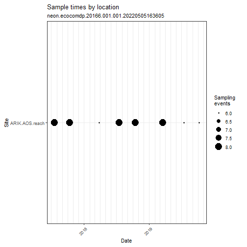
Explore Benthic Algae Data with ecocomDP Plotting Functions

# Note that you can send flattened data 
# to the ecocomDP plotting functions
my_data_benthic %>% ecocomDP::plot_sample_space_time()

# Which taxon ranks are most common?
my_data_benthic %>% ecocomDP::plot_taxa_rank()

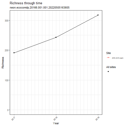
# plot richness by year
my_data_benthic %>% ecocomDP::plot_taxa_diversity(time_window_size = "year")

Check for duplicate taxon counts within a sampleID

# Note that for this data product
# neon_sample_id = event_id
# event_id is a grouping variable for the observation 
# table in the ecocomDP data model



# Check for multiple taxon counts per taxon_id by 
# event_id. 
my_data_benthic %>% 
  group_by(event_id, taxon_id) %>%
  summarize(n_obs = length(event_id)) %>%
  dplyr::filter(n_obs > 1)

## # A tibble: 129 x 3
## # Groups:   event_id [26]
##    event_id                  taxon_id       n_obs
##    <chr>                     <chr>          <int>
##  1 ARIK.20170718.EPIPHYTON.2 NEONDREX1010       2
##  2 ARIK.20170718.EPIPHYTON.2 NEONDREX1024       2
##  3 ARIK.20170718.EPIPHYTON.2 NEONDREX110005     2
##  4 ARIK.20170718.EPIPHYTON.2 NEONDREX155017     2
##  5 ARIK.20170718.EPIPHYTON.2 NEONDREX16004      2
##  6 ARIK.20170718.EPIPHYTON.2 NEONDREX16011      2
##  7 ARIK.20170718.EPIPHYTON.2 NEONDREX170133     2
##  8 ARIK.20170718.EPIPHYTON.2 NEONDREX170134     2
##  9 ARIK.20170718.EPIPHYTON.2 NEONDREX172001     2
## 10 ARIK.20170718.EPIPHYTON.2 NEONDREX172006     2
## # ... with 119 more rows

# Per instructions from the lab, these 
# counts should be summed.
my_data_summed <- my_data_benthic %>%
  group_by(event_id,taxon_id) %>%
  summarize(value = sum(value, na.rm = FALSE),
            observation_id = dplyr::first(observation_id))

my_data_cleaned <- my_data_benthic %>%
  dplyr::select(
    event_id, location_id, datetime,
    taxon_id, taxon_rank, taxon_name) %>%
  distinct() %>%
  right_join(my_data_summed)



# check for duplicate records, there should not 
# be any at this point.
my_data_cleaned %>% 
  group_by(event_id, taxon_id) %>%
  summarize(n_obs = length(event_id)) %>%
  dplyr::filter(n_obs > 1)

## # A tibble: 0 x 3
## # Groups:   event_id [0]
## # ... with 3 variables: event_id <chr>, taxon_id <chr>, n_obs <int>

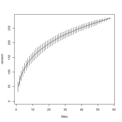
Species Accumulation Curve

Next, we will plot the species accumulation curve for these samples. To do so, we will first need to convert the density data from m2 to cm2, and make the data 'wide':

# convert densities from per m2 to per cm2
my_data_long <- my_data_cleaned %>%
  filter(taxon_rank == "species") %>%
  select(event_id, taxon_id, value)

# make data wide
my_data_wide <- my_data_long %>% 
  pivot_wider(names_from = taxon_id, 
              values_from = value,
              values_fill = list(value = 0)) %>%
  tibble::column_to_rownames("event_id")
  
# Calculate and plot species accumulcation curve for the 11 sampling events
# The CIs are based on random permutations of observed samples
alg_spec_accum_result <- my_data_wide %>% vegan::specaccum(., "random")
plot(alg_spec_accum_result)

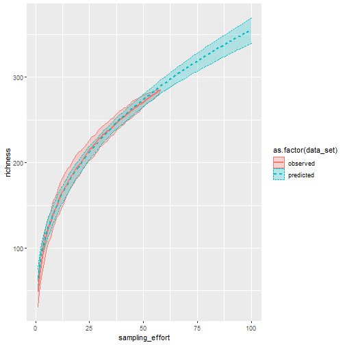
Compare Observed and Simulated species accumulation curves

# Extract the resampling data used in the above algorithm
spec_resamp_data <- data.frame(
  data_set = "observed", 
  sampling_effort = rep(1:nrow(alg_spec_accum_result$perm), 
                        each = ncol(alg_spec_accum_result$perm)),
  richness = c(t(alg_spec_accum_result$perm)))


# Fit species accumulation model
spec_accum_mod_1 <- my_data_wide %>% vegan::fitspecaccum(model = "arrh")


# create a "predicted" data set from the model to extrapolate out 
# beyond the number of samples collected
sim_spec_data <- data.frame()
for(i in 1:100){
  d_tmp <- data.frame(
    data_set = "predicted",
    sampling_effort = i,
    richness = predict(spec_accum_mod_1, newdata = i))
  
  sim_spec_data <- sim_spec_data %>%
    bind_rows(d_tmp)
}


# plot the "observed" and "simulated" curves with 95% CIs
data_plot <- spec_resamp_data %>% bind_rows(sim_spec_data) 

data_plot %>%
  ggplot(aes(sampling_effort, richness, 
             color = as.factor(data_set),
             fill = as.factor(data_set),
             linetype = as.factor(data_set))) +
  stat_summary(fun.data = median_hilow, fun.args = list(conf.int = .95), 
               geom = "ribbon", alpha = 0.25) +
  stat_summary(fun.data = median_hilow, geom = "line", 
               size = 1)