Tutorial
Detecting changes in vegetation structure following fires using discrete-return LiDAR
Authors: Shashi Konduri
Last Updated: Mar 22, 2024
The Creek Fire was a large wildfire that started in September 2020 in the Sierra National Forest, California and became one of the largest fires of the 2020 California wildfire season. This fire had burned into NEON's Soaproot Saddle (SOAP) site by mid-September, causing a high intensity burn over much of the site - standing trees became charcoal spires, shrubs and their root systems burned completely, the thick litter layer was incinerated, and the soil severely burned.
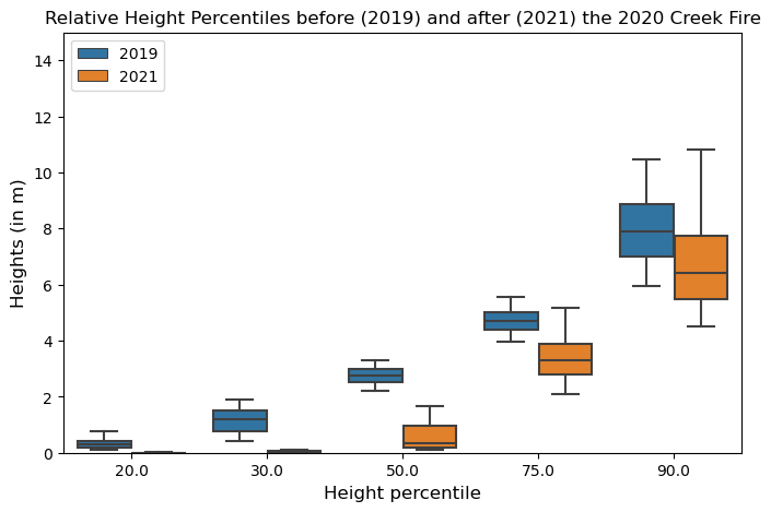
The NEON Airborne Observation Platform (AOP) conducted aerial surveys over SOAP in 2019 and 2021, a year before and after the Creek Fire. This exercise aims to study the effects of fire on vegetation structure by comparing the lidar-derived relative height percentiles before and after the fire. In addition to the discrete return data, this tutorial uses a Digital Terrain Model (DTM) to determine the relative height of the discrete returns with respect to the ground.
This Python tutorial is broken down into three parts:
- Read the NEON discrete-return lidar data (DP1.30003.001) and visualize the 3D lidar point cloud.
- Read the lidar-derived Digital Terrain Model (DP3.30024.001) in Python. Visualize the spatial extent of the lidar data used in this tutorial with that of the Creek Fire perimeter and the SOAP flight boundary.
- Calculate and compare the relative height percentiles of the discrete returns before and after the 2020 Creek Fire.
NEON provides both discrete return and full-waveform LiDAR data for its field sites across the US. The discrete return LiDAR point cloud differs from the full waveform data as it is considerably smaller in file size and condenses the information into a small number of points per laser shot rather than many data bins (roughly 100 bins per laser shot in the full waveform data).
Other NEON tutorials on the use of discrete-return lidar
- If you're interested in using the NEON API to download lidar data using just a few lines of code, please refer to this python tutorial.
- For a more general indroduction to lidar and how to process lidar data in R, please follow this R Tutorial series.
Required resources for this tutorial
The tutorial pre-requisites, the IPython Notebook code, and the datasets used in this tutorial are available on this Google Drive link. The pdf file on tutorial prerequisites goes over the instructions for installing the Anaconda distribution of Python and QGIS. You could also run this tutorial on Google Colab if you do not wish to install Python on your local machine. The subfolder named "NEON_lidar_tutorial_datasets" has shapefiles for the 2020 Creek Fire perimeter, a kml file for the Soaproot site boundary, discrete-return lidar data for the years 2019 and 2021 in .laz format for a small fire-affected area within the SOAP site, and DTM data in .tif format for the same location. The unzipped folder is about 114 MB in size. The shapefile for the 2020 Creek Fire perimeter used in this tutorial was downloaded from the California Department of Forestry and Fire Protection (CAL FIRE) website. It takes about 10 - 15 minutes to execute the code in this Jupyter Notebook depending on whether you run the code locally on your machine or on Google Colab.
Starting the Jupyter Notebook on your local machine
You can launch the Jupyter Notebook by going to the Start Menu and selecting "Jupyter Notebook" under "Anaconda3". Another way is to open a terminal window and run the command "jupyter notebook". This will instantiate a local server on your browser. Click on the "New" dropdown list in the top right corner and select Notebook. This should start an IPython Notebook kernel.
Starting a Google Colab instance
If you prefer using Colab instead, click on "New Notebook". You will have to login to your Google Account. Once the login is successful, it should launch a Colab instance. Every Google Colab instance provides 12 GB RAM usage for free!
Set up the working directory
First, download the Google Drive folder to your local machine by clicking on "Download all", as shown in the screenshot. This will download a zipped file that must be extracted. Make sure the extracted folder's name is "NEON_lidar_tutorial".
1. If you're using Jupyter Notebook on local machine
The code snippet in the cell below will set the working directory as "NEON_lidar_tutorial_datasets" in the Downloads directory. You can execute a code cell by pressing the "Shift + Enter" keys.
import os
home = os.path.expanduser("~")
downloads_path = home + os.sep + "Downloads"
data_root_dir = os.path.join(downloads_path, "NEON_lidar_tutorial", "NEON_lidar_tutorial_datasets")
Note: If you move the data to a different location, you must change the data root directory variable (data_root_dir) to the new directory.
2. If you're using Google Colab
If you are using Google Colab, you can upload the Jupyter Notebook code (fire_effects_on_veg_structure_using_lidar.ipynb) stored locally in the "NEON_lidar_tutorial" folder by selecting "File" --> "Upload Notebook", as shown in the screenshot.
In order to access your datasets from Colab, you can first upload the "NEON_lidar_tutorial" folder to your Google Drive. You can then mount the Google Drive on Colab by clicking on the "Files" icon on the left followed by clicking on the "Mount Drive" icon, as shown in this screenshot.
Note: When using Colab, the data_root_dir defined above would be different. Once you have uploaded the "NEON_lidar_tutorial" folder to your Google Drive and mounted the drive on Colab, you can walk through the directories to get to "NEON_lidar_tutorial_datasets", as shown in this screenshot. You can get the path for this folder by right clicking on the "NEON_lidar_tutorial_datasets" folder --> "Copy Path" and set the data_root_dir variable to that path.
If you are using Colab, uncomment the cell below and run it. Make sure that the path to "NEON_lidar_tutorial_datasets" is correct.
## data_root_dir = "/content/drive/MyDrive/NEON_lidar_tutorial/NEON_lidar_tutorial_datasets/"
Install Python packages
Packages used
- rasterio & rioxarray for reading and plotting raster data
- geopandas for reading shapefiles and kml
- laspy for reading lidar point cloud
- pyproj to change map projections
- shapely to create vector polygons
- seaborn for making boxplots and histograms
To install each of these Python packages from within the Jupyter Notebook, run the command "!pip install" followed by the package's name. Installing all the packages should typically take less than a minute. In a Jupyter Notebook environment, the exclamation mark (!) allows users to run shell commands inside the cell. You'll have to run the following cell only once to install the packages onto your machine. You can suppress the output of a code cell by right clicking on the code cell followed by clicking on "Clear Cell Output".
!pip install rasterio
!pip install rioxarray
!pip install laspy[lazrs,laszip]
!pip install pyproj
!pip install shapely
!pip install seaborn
!pip install geopandas
Now that the packages have been installed, let us import them into the Jupyter Notebook
import pandas as pd
import numpy as np
import laspy, glob, os
import matplotlib.pyplot as plt
from matplotlib.lines import Line2D
from matplotlib.patches import Patch
from mpl_toolkits.mplot3d import axes3d
import pyproj
from pyproj import Proj
import shapely
from shapely import Polygon, MultiPolygon  ## Try this if this line throws an error: from shapely.geometry import Polygon, MultiPolygon
import seaborn as sns
import rasterio
import rioxarray
import geopandas as gpd
from rasterio.plot import show
import random
#import warnings
#warnings.filterwarnings('ignore')
Part 1: Reading and visualizing discrete return lidar data
Read las files in python
Set "Discrete_return_lidar_returns" as the working folder and import the point cloud data for 2019 and 2021.
# define the discrete_lidar_directory and change into that directory to read in the point cloud files
discrete_lidar_dir = os.path.join(data_root_dir,"Discrete_return_lidar_returns")
os.chdir(discrete_lidar_dir)

las_2021 = laspy.read("NEON_D17_SOAP_DP1_293000_4100000_classified_point_cloud_colorized_2021.laz")
las_2019 = laspy.read("NEON_D17_SOAP_DP1_293000_4100000_classified_point_cloud_colorized_2019.laz")

## Print all the fields provided by the las files
print(list(las_2021.point_format.dimension_names))
['X', 'Y', 'Z', 'intensity', 'return_number', 'number_of_returns', 'synthetic', 'key_point', 'withheld', 'overlap', 'scanner_channel', 'scan_direction_flag', 'edge_of_flight_line', 'classification', 'user_data', 'scan_angle', 'point_source_id', 'gps_time', 'red', 'green', 'blue']
Read point cloud data as a dataframe
The "las_to_df" function defined below imports the .las file as a Python dataframe. For more information about the las format, please refer to the ASPRS documentation. Las files provide the following information:
- X, Y, and Z (height above vertical datum) coordinates of the discrete return.
- Intensity of the return. In discrete-return lidar, laser pulses that reflect off single return objects, such as the ground have a much higher intensity than pulses that must penetrate the canopy (which lose photon energy with each interaction).
- Return number and total number of returns per pulse. Each lidar pulse can have multiple returns along the vertical profile. The first return typically comes from the top of the canopy, while the last return tends to be from the ground.
- Classification of the return. Lastools software follows the standard ASPRS classification scheme to classify returns as ground, low vegetation, high vegetation, buildings, etc.
- Scan angle of the lidar sensor at which the return was collected (can vary from -18 degrees to + 18 degrees). This information could be used to drop returns collected at extreme values of scan angle.
For more information about how the NEON lidar point cloud data were created, refer to the NEON L0-to-L1 Discrete Return LiDAR Algorithm Theoretical Basis Document (ATBD) found on the NEON data product page.
## Function to import las file as a dataframe in python
def las_to_df(las):
  x = pd.DataFrame(np.array(las.x))
  y = pd.DataFrame(np.array(las.y))
  z = pd.DataFrame(np.array(las.z))
  intensity = pd.DataFrame(np.array(las.intensity))
  return_num = pd.DataFrame(np.array(las.return_number))
  number_of_returns = pd.DataFrame(np.array(las.number_of_returns))
  classification = pd.DataFrame(np.array(las.classification)) ## 0 - 31 as per ASPRS classification scheme

  df = pd.concat([x, y, z, intensity, return_num, number_of_returns, classification], axis=1)
  df.columns=["x", "y", "z", "intensity", "return_num", "number_of_returns", "classification"]
  return(df)
## Call the las_to_df function to extract the 2019 and 2021 data as separate dataframes
point_cloud_df_2019 = las_to_df(las_2019)
point_cloud_df_2021 = las_to_df(las_2021)
point_cloud_df_2021.head()
| x | y | z | intensity | return_num | number_of_returns | classification | |
|---|---|---|---|---|---|---|---|
| 0 | 293396.362 | 4100000.012 | 907.778 | 25 | 3 | 3 | 2 |
| 1 | 293396.347 | 4100000.014 | 907.762 | 27 | 3 | 3 | 2 |
| 2 | 293396.324 | 4100000.019 | 907.710 | 32 | 3 | 3 | 2 |
| 3 | 293396.336 | 4100000.016 | 907.754 | 36 | 3 | 3 | 2 |
| 4 | 293396.323 | 4100000.019 | 907.714 | 36 | 3 | 3 | 2 |
The X and Y output coordinates are reported as Easting and Northing values in a Universal Transverse Mercator (UTM) projection with the World Geodetic System 1984 (WGS84) International Terrestrial Reference Frame 2000 (ITRF 2000) ellipsoid horizontal datum with units of meters. The UTM zone will vary depending on the latitude/longitude of the specific NEON site. The Z coordinates are reported in a North American Vertical Datum 1988 (NAVD88) using the National Geodetic Survey Geoid12A height model with units of meters. For a gentle introduction to reference datums and projection systems, please refer to this article.
For the Z values to make more sense, we will use the ground elevations from a Digital Terrain Model (DTM) to calculate the height of the discrete returns relative to the ground.
Create 3D visualization of discrete-return point cloud
Before we get to calculating the heights of each return with respect to ground, we'll visualize the discrete returns in three dimensions. To visualize the 3D point cloud data, we first combine the X, Y, and Z dimensions using the numpy package (abbreviated here as np). We then plot the X, Y, and Z values for each discrete return and colorize each return with its R, G, and B values.
## Use np.stack to combine the X, Y and Z into one array
## Convert (3 x n) array to (n x 3) using transpose
point_data_2021 = np.stack([las_2021.X, las_2021.Y, las_2021.Z]).transpose()
point_data_2019 = np.stack([las_2019.X, las_2019.Y, las_2019.Z]).transpose()
print("Number of discrete returns in the 2021 point cloud file = %s" %"{:,}".format(point_data_2021.shape[0]))
print("Number of discrete returns in the 2019 point cloud file = %s" %"{:,}".format(point_data_2019.shape[0]))
Number of discrete returns in the 2021 point cloud file = 15,278,262
Number of discrete returns in the 2019 point cloud file = 3,015,329
Since the point cloud files have millions of discrete returns, plotting them will take a substantial amount of time (~15-20 minutes). To avoid spending a lot of time, we will sample a small fraction of them. In the code below, we will sample every 100th return for plotting.
factor=100
point_data_2021_sub = point_data_2021[::factor]
point_data_2019_sub = point_data_2019[::factor]
print("Number of discrete returns in the 2021 point cloud subsample = %s" %"{:,}".format(point_data_2021_sub.shape[0]))
print("Number of discrete returns in the 2019 point cloud subsample = %s" %"{:,}".format(point_data_2019_sub.shape[0]))
Number of discrete returns in the 2021 point cloud subsample = 152,783
Number of discrete returns in the 2019 point cloud subsample = 30,154
Now, we will extract the Red (R), Green (G), and Blue (B) values associated with each discrete return. The RGB data is collected by the camera sensor fitted on the airplane. Think of this as "draping" the camera imagery on top of the lidar discrete returns, so we have additional context when plotting the returns.
colors_2021 = np.stack([las_2021.red, las_2021.green, las_2021.blue]).transpose()
colors_2019 = np.stack([las_2019.red, las_2019.green, las_2019.blue]).transpose()
The RGB values are coded on 16 bits in the las file, ranging between $2^0$ and $2^{16}$ for each band. We need to scale the RGB color values to lie between 0 and 1 for plotting, thus, we are going to subtract the min(band value) and divide by the range of band values.
colors_2021_normalized = (colors_2021 - np.min(colors_2021))/np.ptp(colors_2021)
colors_2021_normalized_sub = colors_2021_normalized[::factor]
## We are going to zip the R,G,B values together for plotting using the matplotlib package
colors_2021_normalized_sub = list(zip(colors_2021_normalized_sub[:,0], colors_2021_normalized_sub[:,1], colors_2021_normalized_sub[:,2]))

colors_2019_normalized = (colors_2019 - np.min(colors_2019))/np.ptp(colors_2019)
colors_2019_normalized_sub = colors_2019_normalized[::factor]
colors_2019_normalized_sub = list(zip(colors_2019_normalized_sub[:,0], colors_2019_normalized_sub[:,1], colors_2019_normalized_sub[:,2]))
Now, we will plot the x, y, and z coordinates of every discrete return sampled from 2021 and colorize them using the RGB value from the camera sensor.
# Plot the las data in 3D
fig = plt.figure(figsize=(6,6))
ax = fig.add_subplot(111, projection='3d')

## Plot the 2021 data
ax.scatter(point_data_2021_sub[:,0], point_data_2021_sub[:,1], point_data_2021_sub[:,2], color=colors_2021_normalized_sub, s=4)
plt.show()
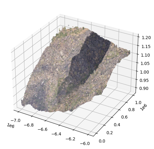
The dark shade in the middle is a cloud shadow. We will now make a similar plot for returns sampled from 2019
fig = plt.figure(figsize=(6,6))
ax = fig.add_subplot(111, projection='3d')
ax.scatter(point_data_2019_sub[:,0], point_data_2019_sub[:,1], point_data_2019_sub[:,2], color=colors_2019_normalized_sub, s=4)
plt.show()
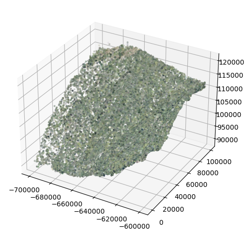
Visually comparing the randomly-sampled colorized point clouds from the two years reveals burn scars with gaps in vegetation in 2021 relative to 2019.
Part 2: Ingest and visualize the Digital Terrain Model (DTM)
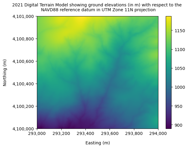
Next, we'll explore a Python library called rioxarray for reading and plotting raster data. The rioxrray object has metadata information stored in the tiff tags. The DTM files are provided as 1 x 1 km tiles at a 1-m spatial resolution, which is why the resulting dataframe is of size 1000 x 1000.
os.chdir(os.path.join(data_root_dir,"Digital_Terrain_Model"))
dtm_2021 = rioxarray.open_rasterio("NEON_D17_SOAP_DP3_293000_4100000_DTM_2021.tif")
dtm_2019 = rioxarray.open_rasterio("NEON_D17_SOAP_DP3_293000_4100000_DTM_2019.tif")
print(dtm_2021)
<xarray.DataArray (band: 1, y: 1000, x: 1000)>
[1000000 values with dtype=float32]
Coordinates:
  * band         (band) int32 1
  * x            (x) float64 2.93e+05 2.93e+05 2.93e+05 ... 2.94e+05 2.94e+05
  * y            (y) float64 4.101e+06 4.101e+06 4.101e+06 ... 4.1e+06 4.1e+06
    spatial_ref  int32 0
Attributes: (12/14)
    AREA_OR_POINT:             Area
    TIFFTAG_ARTIST:            Created by the National Ecological Observatory...
    TIFFTAG_COPYRIGHT:         The National Ecological Observatory Network is...
    TIFFTAG_DATETIME:          Flown on 2021071215, 2021071315-P1C2
    TIFFTAG_IMAGEDESCRIPTION:  Elevation LiDAR - NEON.DP3.30024 acquired at S...
    TIFFTAG_MAXSAMPLEVALUE:    1187
    ...                        ...
    TIFFTAG_SOFTWARE:          Tif file created with a Matlab script (write_g...
    TIFFTAG_XRESOLUTION:       1
    TIFFTAG_YRESOLUTION:       1
    _FillValue:                -9999.0
    scale_factor:              1.0
    add_offset:                0.0
You can expand the information stored in the specific attributes by using the 'attrs' keyword.
print("****2021 DTM Metdata******")
print(dtm_2021.attrs["TIFFTAG_IMAGEDESCRIPTION"])

print("****2019 DTM Metdata******")
print(dtm_2019.attrs["TIFFTAG_IMAGEDESCRIPTION"])
****2021 DTM Metdata******
Elevation LiDAR - NEON.DP3.30024 acquired at SOAP by Teledyne Optech Galaxy Prime 5060445 as part of P1C2
****2019 DTM Metdata******
Elevation LiDAR - NEON.DP3.30024 acquired at SOAP by Optech, Inc Gemini 12SEN311 as part of P2C1
As per the information provided in the 'TIFFTAG_IMAGEDESCRIPTION' field in the metadata, it can be seen that NEON flew the older Optech Gemini lidar sensor in 2019 and the new Optech Galaxy Prime sensor in 2021. When comparing lidar data collected across different years, it is essential to check if the lidar sensors used for the collections are consistent. Older sensors like the Optech Gemini have a wider outgoing pulse width, resulting in poorer range resolution than the newer Optech Galaxy Prime. Poor range resolution for a lidar sensor makes it challenging to resolve objects close to the ground (such as low vegetation). Optech Gemini has a range resolution of about 2 m, which means it can be challenging to distinguish objects less than 2 m apart along the vertical profile. The range resolution for the newer Optech Galaxy Prime is substantially better, at around 67 cm. For more information on range resolution for NEON lidar sensors, please refer to section 4.1.1.3 of the NEON Algorithm Theoretical Basis Document (ATBD) for the discrete-return data. We can extract the ground elevations form the DTM raster as follows:
## Extract the DTM data, which is stored in band 1
dtm_2021_data = dtm_2021.data[0,:,:]

## Print the values stored in the DTM dataframe
print(dtm_2021_data)
[[1130.147 1130.136 1130.13  ... 1110.648 1109.383 1109.14 ]
 [1130.048 1130.04  1129.988 ... 1109.33  1109.154 1109.173]
 [1130.032 1129.989 1129.85  ... 1109.293 1108.92  1108.888]
 ...
 [ 898.096  897.757  897.339 ... 1048.097 1048.502 1048.752]
 [ 897.679  897.366  896.929 ... 1047.965 1048.324 1048.595]
 [ 897.246  896.993  896.586 ... 1047.734 1048.132 1048.418]]
The values stored in the DTM dataframe are ground elevations (in m) with respect to the NAVD88 reference datum.
dtm_2021.plot()
plt.title("2021 Digital Terrain Model showing ground elevations (in m) with respect to the \n NAVD88 reference datum in UTM Zone 11N projection", fontsize=10, pad=12)
plt.ylabel("Northing (m)", labelpad=12)
plt.xlabel("Easting (m)", labelpad=12)

xticks = np.arange(293000, 294200, 200)
comma_sep_xticks = []
for num in xticks:
   comma_sep_num = "{:,}".format(num)
   comma_sep_xticks.append(comma_sep_num)

yticks = np.arange(4100000,4101200,200)
comma_sep_yticks = []
for num in yticks:
   comma_sep_num = "{:,}".format(num)
   comma_sep_yticks.append(comma_sep_num)

plt.xticks(xticks, comma_sep_xticks)
plt.yticks(yticks, comma_sep_yticks)

plt.show()
Optional: Visualize the relative spatial extent of the lidar data used in relation to the Creek Fire perimeter
You can skip this section and go straight to Part 3, as it is not key to this tutorial. Here, we will use the Python packages geopandas for ingesting vector data and matplotlib to plot the spatial extent of the 2020 Creek fire relative to that of the NEON site at Soaproot Saddle (SOAP). Geopandas is a popular Python package for handling vector data, such as shapefiles and kml files. The SOAP boundary file is provided in kml format, whereas the Creek fire extent is available as a shapefile. You will also notice that these files are available in different projections, which prevents us from plotting them on the same axis. Projection information is usually provided as a unique four-digit EPSG code and can be accessed from a Geopandas object using the keyword "crs". You may refer to this article again for more information on EPSG codes 3857 and 4326.
## Go inside the creek fire boundary subfolder and ingest the shape file
os.chdir(os.path.join(data_root_dir,"Creek_fire_boundary"))
creek_fire_perimeter = gpd.read_file("creek_fire_perimeter.shp")
creek_fire_perimeter.plot(color='red', figsize=(3.5,5))
plt.ylabel("Northing", labelpad=12)
plt.xlabel("Easting", labelpad=12)
plt.show()
print("Projection for creek fire shapefile = %s" %creek_fire_perimeter.crs)

## Now go into the Soaproot site boundary subfolder and ingest the kml file
os.chdir(os.path.join(data_root_dir,"SOAP_site_boundary"))
#gpd.io.file.fiona.drvsupport.supported_drivers['KML'] = 'rw'  ## you might need this to enable geopandas to read a kml file
soap_boundary = gpd.read_file("NEON_D17_SOAP_DPQA_2021_full_boundary.kml", driver='KML')
soap_boundary.plot(color="yellow", figsize=(3,3))
plt.ylabel("Latitude", labelpad=12)
plt.xlabel("Longitude", labelpad=12)
plt.show()
print("Projection for Soaproot Saddle kml file = %s" %soap_boundary.crs)
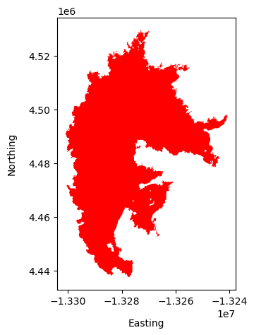
Projection for creek fire shapefile = EPSG:3857
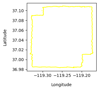
Projection for Soaproot Saddle kml file = EPSG:4326
Maps are usually provided in different projections, and converting from one to another is common. Here, we will convert the Creek Fire shapefile from EPSG:3857 to 4326 using the Pyproj package. Since the Creek fire shapefile is a collection of polygons, the coordinates for each of the polygon need to converted from EPSG:3857 to 4326. The following code cell demonstrates how this conversion works for one polygon.
## Save the Creek fire polygons as a list
multipolygons = list(creek_fire_perimeter["geometry"][0].geoms)

## Print the first polygon from the multi polygons list
index=0
print(multipolygons[index])

## Extract the x and y for the first polygon
y = list(multipolygons[index].exterior.coords.xy[0])
x = list(multipolygons[index].exterior.coords.xy[1])

## Create projection objects for the source and target projections
epsg_3857 = Proj(projparams = 'epsg:3857')
epsg_4326 = Proj(projparams = 'epsg:4326')

## Transform coordinates from EPSG:3857 to EPSG:4326
latlons = Polygon(list(zip(pyproj.transform(epsg_3857, epsg_4326, y, x)[0], pyproj.transform(epsg_3857, epsg_4326, y, x)[1])))
print(latlons)
POLYGON ((-13267204.057 4452524.504000001, -13267209.1792 4452516.816799998, -13267214.9785 4452521.142899998, -13267219.1984 4452525.169699997, -13267216.2523 4452528.064800002, -13267212.2181 4452534.154700004, -13267209.2986 4452533.322800003, -13267206.6843 4452528.796899997, -13267204.057 4452524.504000001))
POLYGON ((37.09620129816644 -119.1813218193562, 37.09614621799331 -119.1813678328617, 37.09617721528422 -119.18141992886, 37.09620606802497 -119.1814578368667, 37.09622681192648 -119.1814313716001, 37.09627044711418 -119.1813951317649, 37.09626448640815 -119.1813689054502, 37.096232057551 -119.1813454207937, 37.09620129816644 -119.1813218193562))
We will now run a for loop to reproject the coordinates of all polygons in the creek fire shapefile
multipolygon_latlon_list = []

for index in range(0, len(multipolygons)):
    ## Extract the x and y for the polygon
    y = list(multipolygons[index].exterior.coords.xy[0])
    x = list(multipolygons[index].exterior.coords.xy[1])
    multipolygon_latlon_list.append(Polygon(list(zip(pyproj.transform(epsg_3857, epsg_4326, y, x)[1], pyproj.transform(epsg_3857, epsg_4326, y, x)[0]))))

## Update the geometry information in the creek fire perimeter
creek_fire_perimeter["geometry"][0] = MultiPolygon(multipolygon_latlon_list)
We can also plot the extent of 2021 DTM, which is available in yet another projection, UTM Zone 11N. We will again use the Pyproj package to convert the UTM coordinates of the DTM bounding box to lat lon. Then we will use the Shapely package to create a polygon whose corners are the lat/lon values of the DTM bounding box.
os.chdir(os.path.join(data_root_dir,"Digital_Terrain_Model"))
dtm_2021 = rasterio.open("NEON_D17_SOAP_DP3_293000_4100000_DTM_2021.tif")
dtm_2019 = rasterio.open("NEON_D17_SOAP_DP3_293000_4100000_DTM_2019.tif")

## Convert UTM coordinates of the DTM bounding box to lat/lon
utm_proj = Proj("+proj=utm +zone=11 +north +ellps=WGS84 +datum=WGS84 +units=m")
lon_min, lat_min = utm_proj(dtm_2021.bounds[0], dtm_2021.bounds[1], inverse=True)
lon_max, lat_max = utm_proj(dtm_2021.bounds[2], dtm_2021.bounds[3], inverse=True)

corner_coords = [[lon_min, lat_min], [lon_min, lat_max], [lon_max, lat_max], [lon_max, lat_min]]

## Create a shapely polygon using corner lat/lons
polygon_geometry = Polygon(corner_coords)
df = {'Attribute':['DTM_extent'], 'geometry':polygon_geometry} # create a dictionary with needed attributes
dtm_polygon = gpd.GeoDataFrame(df, geometry='geometry', crs='EPSG:4326')
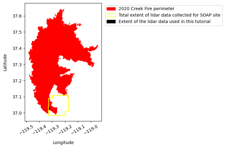
Let's plot the spatial extent of the creek fire, Soaproot saddle site (SOAP) boundary, and the 1 x 1 km 2021 DTM raster together, now that they are all in lat/lon.
creek_fire = creek_fire_perimeter.plot(color='red', figsize=(5,5))
soap_boundary.plot(ax=creek_fire, color='yellow')
dtm_polygon.plot(ax=creek_fire, color='black')
plt.ylabel("Latitude", labelpad=12)
plt.xlabel("Longitude", labelpad=12)
plt.xticks(rotation=30)

## Add legend
legend_elements = [Patch(facecolor='red', edgecolor='red', label='2020 Creek Fire perimeter'),
                  Patch(facecolor='none', edgecolor='yellow', label='Total extent of lidar data collected for SOAP site'),
                  Patch(facecolor='black', edgecolor='black', label='Extent of the lidar data used in this tutorial')]
plt.legend(handles=legend_elements, bbox_to_anchor=(2.6,1))
plt.show()
Part 3: Calculate and compare the relative height percentiles of the discrete returns before (2019) and after (2021) the 2020 Creek fire.
We will now be calculating pixel-wise height percentiles ($20^{th}$, $30^{th}$, $50^{th}$, $75^{th}$, and $90^{th}$ percentile heights) of the discrete returns relative to the ground (DTM) for the years 2019 and 2021. To ensure that we have sufficient number of lidar returns per pixel for calculating percentiles, we will be calculating these metrics for every 10m pixel on the ground. So, our tasks here would be to:
- Calculate heights of discrete returns with repect to the 1m DTM. Since the ground heights do not change from year to year, we will be using the 2021 DTM to calculate heights of the discrete returns with respect to ground for both the years 2019 and 2021. The 2020 fire event would have likely cleared up some of the low vegetation and ground litter, thereby improving ground detection post-fire in 2021. Therefore, the 2021 DTM may be a more accurate representation of the true ground compared to the 2019 DTM.
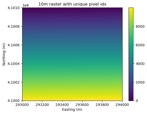
- Create a 10m spatial resolution raster grid and assign a unique id to each 10m pixel.
- Group all discrete returns based on the 10m pixel they fall into.
- Calculate height percentiles ($20^{th}$, $30^{th}$, $50^{th}$, $75^{th}$, and $90^{th}$ percentile heights) relative to the ground for each 10m pixel.
- Compare the distribution of heights for each height percentile before and after the fire.
1. Discrete-return heights relative to 2021 DTM
To extract the ground elevation associated with each discrete return, we will be sampling values from the 2021 DTM raster at the x,y locations of each discrete return. We can then subtract the ground elevation from the height of the discrete return (z) to get the height of the return above ground.
## zip all x and y coordinates together for sampling rasters in the next cell
coords_2019 = [(x,y) for x, y in zip(point_cloud_df_2019["x"], point_cloud_df_2019["y"])]
coords_2021 = [(x,y) for x, y in zip(point_cloud_df_2021["x"], point_cloud_df_2021["y"])]

print("Number of discrete returns in 2021 data = %d" %len(coords_2021))
print("Number of discrete returns in 2019 data = %d" %len(coords_2019))
Number of discrete returns in 2021 data = 15278262
Number of discrete returns in 2019 data = 3015329
As you can see, there are about 15 million discrete returns in the 2021 point cloud data compared to the roughly 3 million returns in the 2019 data. The difference in the # of returns can be attributed to the different sensors used in the two years. Sampling the ground elevations for all these returns would take several minutes. In the next cell, we are going to sample 1 million returns randomly for 2019 and 2021. Extracting the ground elevations for these million returns for both years would take about 2 minutes.
## Set a seed value to make the code output reproducible
seed_val = 0
random.seed(seed_val)

## Randomly sample 1 million rows from the 2019 and 2021 point cloud dataframes
point_cloud_df_2019_sub = point_cloud_df_2019.sample(n=1000000).reset_index(drop=True)
point_cloud_df_2021_sub = point_cloud_df_2021.sample(n=1000000).reset_index(drop=True)

## zip all x and y coordinates together for sampling rasters in the next step
coords_2019_sub = [(x,y) for x, y in zip(point_cloud_df_2019_sub["x"], point_cloud_df_2019_sub["y"])]
coords_2021_sub = [(x,y) for x, y in zip(point_cloud_df_2021_sub["x"], point_cloud_df_2021_sub["y"])]

## Sample the raster using "rasterio.sample.sample_gen()"

## Sample the 2021 DTM raster for ground elevation at each (x,y) location of the 2021 discrete returns
dtm_vals_2021 = pd.DataFrame(list(rasterio.sample.sample_gen(dtm_2021, coords_2021_sub)))

## Sample the 2021 DTM raster for ground elevation at each (x,y) location of the 2019 discrete returns
## The ground elevations shouldn't change from year to year, so it is OK to use the 2021 DTM for both years.
## Moreover, the fire event in 2020 likely cleared the understory vegetation, and therefore, the ground elevations might be more accurate in 2021
dtm_vals_2019 = pd.DataFrame(list(rasterio.sample.sample_gen(dtm_2021, coords_2019_sub)))
## Merge the point cloud dataframe (point_cloud_df_20xx_sub) with the DTM ground elevations extracted (dtm_vals_20xx)
## Calculate the relative height of each return with respect to ground ("discrete_ret_ht_above_ground")

## 2019
df_2019 = pd.concat([point_cloud_df_2019_sub, dtm_vals_2019], axis=1)
df_2019.columns = ["x", "y", "z", "intensity", "return_num", "number_of_returns", "classification", "ground_elevation"]
df_2019["discrete_ret_ht_above_ground"] = df_2019["z"] - df_2019["ground_elevation"]

## Do the same for 2021 data as well
df_2021 = pd.concat([point_cloud_df_2021_sub, dtm_vals_2021], axis=1)
df_2021.columns = ["x", "y", "z", "intensity", "return_num", "number_of_returns", "classification", "ground_elevation"]
df_2021["discrete_ret_ht_above_ground"] = df_2021["z"] - df_2021["ground_elevation"]
df_2021.head()
| x | y | z | intensity | return_num | number_of_returns | classification | ground_elevation | discrete_ret_ht_above_ground | |
|---|---|---|---|---|---|---|---|---|---|
| 0 | 293456.586 | 4100430.746 | 1047.418 | 46 | 2 | 2 | 2 | 1047.392944 | 0.025056 |
| 1 | 293918.894 | 4100471.724 | 1078.615 | 115 | 2 | 2 | 2 | 1078.479004 | 0.135996 |
| 2 | 293729.187 | 4100541.491 | 1030.690 | 194 | 1 | 1 | 2 | 1030.792969 | -0.102969 |
| 3 | 293781.364 | 4100320.959 | 1033.607 | 32 | 1 | 2 | 1 | 1032.322021 | 1.284979 |
| 4 | 293193.611 | 4100784.243 | 1155.679 | 117 | 3 | 3 | 2 | 1155.823975 | -0.144975 |
2. Create a 10m spatial resolution raster grid and assign a unique id to each 10m pixel
## Save the new 5m raster in the DTM data folder
dtm_directory = os.path.join(data_root_dir,"Digital_Terrain_Model")
os.chdir(dtm_directory)

## Create a (100 x 100) dataframe with each cell having a unique value between 0 and 10,000
ids = pd.DataFrame(data=np.arange(0, 100*100).reshape(100,100), index=np.arange(0,100), columns=np.arange(0,100))

## Create a scaled transform
scaled_transform = dtm_2021.transform * dtm_2021.transform.scale((10),(10))

## Using rasterio, save the dataframe as a 10m raster in the tif format
with rasterio.open(
    dtm_directory + '/DTM_10m_unique_id.tif',
    'w',
    driver='GTiff',
    height=ids.shape[0],
    width=ids.shape[1],
    count=1,
    dtype=np.dtype(np.int32),
    crs=dtm_2021.crs,
    transform=scaled_transform,
) as dst:
    dst.write(ids, 1)
## Use rioxarray again to plot the newly created 10m raster
raster_10m = rioxarray.open_rasterio("DTM_10m_unique_id.tif")
print(raster_10m)
raster_10m.plot()
plt.xlabel("Easting (m)")
plt.ylabel("Northing (m)")
plt.title("10m raster with unique pixel ids")
plt.show()
<xarray.DataArray (band: 1, y: 100, x: 100)>
[10000 values with dtype=int32]
Coordinates:
  * band         (band) int32 1
  * x            (x) float64 2.93e+05 2.93e+05 2.93e+05 ... 2.94e+05 2.94e+05
  * y            (y) float64 4.101e+06 4.101e+06 4.101e+06 ... 4.1e+06 4.1e+06
    spatial_ref  int32 0
Attributes:
    AREA_OR_POINT:  Area
    scale_factor:   1.0
    add_offset:     0.0
3. Group all discrete returns based on the 10m pixel they fall into.
## Here, we assign unique ids created in the previous cell to each discrete return
## Sample the unique ids from the 10m raster for each discrete return for the years 2019 and 2021
## This sampling step might again take a few minutes

raster_10m = rasterio.open("DTM_10m_unique_id.tif")
## For the year 2021
dtm_id_vals_2021 = pd.DataFrame(list(rasterio.sample.sample_gen(raster_10m, coords_2021_sub)))

## For the year 2019
dtm_id_vals_2019 = pd.DataFrame(list(rasterio.sample.sample_gen(raster_10m, coords_2019_sub)))
## Merge the unique ids extracted above with the discrete return dataframe (df_20xx) created earlier

## Update 2019 df
df_2019_with_ids = pd.concat([df_2019, dtm_id_vals_2019], axis=1)
df_2019_with_ids.columns = ["x", "y", "z", "intensity", "return_num", "number_of_returns", "classification",
                   "ground_elevation", "discrete_ret_ht_above_ground", "uniq_id"]
df_2019_with_ids = df_2019_with_ids[df_2019_with_ids["ground_elevation"] > -9999.0].reset_index(drop=True)

## Update 2021 df
df_2021_with_ids = pd.concat([df_2021, dtm_id_vals_2021], axis=1)
df_2021_with_ids.columns = ["x", "y", "z", "intensity", "return_num", "number_of_returns", "classification",
                            "ground_elevation", "discrete_ret_ht_above_ground", "uniq_id"]
df_2021_with_ids = df_2021_with_ids[df_2021_with_ids["ground_elevation"] > -9999.0].reset_index(drop=True)
df_2021_with_ids.head()
| x | y | z | intensity | return_num | number_of_returns | classification | ground_elevation | discrete_ret_ht_above_ground | uniq_id | |
|---|---|---|---|---|---|---|---|---|---|---|
| 0 | 293456.586 | 4100430.746 | 1047.418 | 46 | 2 | 2 | 2 | 1047.392944 | 0.025056 | 5645 |
| 1 | 293918.894 | 4100471.724 | 1078.615 | 115 | 2 | 2 | 2 | 1078.479004 | 0.135996 | 5291 |
| 2 | 293729.187 | 4100541.491 | 1030.690 | 194 | 1 | 1 | 2 | 1030.792969 | -0.102969 | 4572 |
| 3 | 293781.364 | 4100320.959 | 1033.607 | 32 | 1 | 2 | 1 | 1032.322021 | 1.284979 | 6778 |
| 4 | 293193.611 | 4100784.243 | 1155.679 | 117 | 3 | 3 | 2 | 1155.823975 | -0.144975 | 2119 |
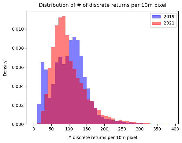
The unique ids in the last column are not ordered as the discrete returns were sampled randomly. Before we calculate the relative height percentiles, let's look at the distribution of the number of discrete returns per 10m pixel for the years 2019 and 2021. A sufficient number of returns per 10m pixel will ensure that the height percentiles are robust.
fig, ax = plt.subplots()
return_counts_per_10m_pixel_2019 = np.unique(df_2019_with_ids["uniq_id"].sort_values(), return_counts=True)[1]
return_counts_per_10m_pixel_2021 = np.unique(df_2021_with_ids["uniq_id"].sort_values(), return_counts=True)[1]
plt.hist(return_counts_per_10m_pixel_2019, bins=np.arange(0,400,10), density=True, alpha=0.5, color="blue")
plt.hist(return_counts_per_10m_pixel_2021, bins=np.arange(0,400,10), density=True, alpha=0.5, color="red")
plt.xlabel("# discrete returns per 10m pixel", labelpad=10)
plt.ylabel("Density", labelpad=10)
plt.title("Distribution of # of discrete returns per 10m pixel", fontsize=12, pad=10)

legend_elements = [Patch(facecolor="blue", edgecolor="blue", label='2019', alpha=0.5),
                  Patch(facecolor="red", edgecolor="red", label='2021', alpha=0.5)]
plt.legend(handles=legend_elements)
plt.show()
4. Calculate height percentiles of discrete returns ($20^{th}$, $30^{th}$, $50^{th}$, $75^{th}$, and $90^{th}$) for each 10m pixel.
Before we calculate the height percentiles, we will drop 10-m pixels with too few discrete returns (< 50).
## Subset the dataframes to include only the relevant columns
df_2019_sub = pd.concat([df_2019_with_ids["x"], df_2019_with_ids["y"], df_2019_with_ids["uniq_id"], df_2019["discrete_ret_ht_above_ground"]], axis=1)
df_2021_sub = pd.concat([df_2021_with_ids["x"], df_2021_with_ids["y"], df_2021_with_ids["uniq_id"], df_2021["discrete_ret_ht_above_ground"]], axis=1)

## Calculate the number of returns per 10 m pixel
return_counts_per_10m_pixel_2019 = pd.DataFrame(np.unique(df_2019_sub["uniq_id"].sort_values(), return_counts=True)).transpose()
return_counts_per_10m_pixel_2021 = pd.DataFrame(np.unique(df_2021_sub["uniq_id"].sort_values(), return_counts=True)).transpose()
return_counts_per_10m_pixel_2019.columns = return_counts_per_10m_pixel_2021.columns = ["uniq_id", "number_of_returns"]

## Select only those 10m pixels which have greater than 50 returns
return_counts_per_10m_pixel_2019 = return_counts_per_10m_pixel_2019[return_counts_per_10m_pixel_2019["number_of_returns"] > 50].reset_index(drop=True)
return_counts_per_10m_pixel_2021 = return_counts_per_10m_pixel_2021[return_counts_per_10m_pixel_2021["number_of_returns"] > 50].reset_index(drop=True)
valid_10m_pixels_2019 = return_counts_per_10m_pixel_2019["uniq_id"]
valid_10m_pixels_2021 = return_counts_per_10m_pixel_2021["uniq_id"]

## Update df_sub to include only valid 10m pixels (returns > 50)
df_2019_sub = df_2019_sub[df_2019_sub["uniq_id"].isin(valid_10m_pixels_2019)].reset_index(drop=True)
df_2021_sub = df_2021_sub[df_2021_sub["uniq_id"].isin(valid_10m_pixels_2021)].reset_index(drop=True)
## For each unique id (uniq_id), calculate relative height percentiles (20th, 30th, 50th, 75th and 90th)

## First define a function to calculate the percentile and return a percentile dataframe
def calc_percentile(df,percentile):
    ptile_df = pd.DataFrame(df.groupby(by=["uniq_id"])["discrete_ret_ht_above_ground"].quantile(percentile).reset_index(drop=True))
    ptile_df["RH_ptile"] = percentile*100
    ptile_df.columns = ["height", "RH_ptile"]
    return ptile_df

ptile_20_2019 = calc_percentile(df_2019_sub,0.2)
ptile_30_2019 = calc_percentile(df_2019_sub,0.3)
ptile_50_2019 = calc_percentile(df_2019_sub,0.5)
ptile_75_2019 = calc_percentile(df_2019_sub,0.75)
ptile_90_2019 = calc_percentile(df_2019_sub,0.9)

ptile_20_2021 = calc_percentile(df_2021_sub,0.2)
ptile_30_2021 = calc_percentile(df_2021_sub,0.3)
ptile_50_2021 = calc_percentile(df_2021_sub,0.5)
ptile_75_2021 = calc_percentile(df_2021_sub,0.75)
ptile_90_2021 = calc_percentile(df_2021_sub,0.9)
Combine these into single dataframes so we can plot all the data together.
rh_percentiles_2019 = pd.concat([ptile_20_2019, ptile_30_2019, ptile_50_2019, ptile_75_2019, ptile_90_2019], axis=0, ignore_index=True)
rh_percentiles_2019["year"] = 2019

rh_percentiles_2021 = pd.concat([ptile_20_2021, ptile_30_2021, ptile_50_2021, ptile_75_2021, ptile_90_2021], axis=0, ignore_index=True)
rh_percentiles_2021["year"] = 2021

## Combine 2019 and 2021 dataframes
rh_percentiles_combined = pd.concat([rh_percentiles_2019, rh_percentiles_2021], axis=0, ignore_index=True)
5. Compare the distribution of height percentiles for the years 2019 and 2021.
## Compare boxplots
plt.subplots(figsize=(8,5))
sns.boxplot(x=rh_percentiles_combined["RH_ptile"], y=rh_percentiles_combined["height"], hue=rh_percentiles_combined["year"],
           fliersize=0, whis=[5,95])
plt.ylim(0,15)
plt.xlabel("Height percentile", fontsize=12)
plt.ylabel("Heights (in m)", fontsize=12)
plt.title("Relative Height Percentiles before (2019) and after (2021) the 2020 Creek Fire")
plt.legend(loc='upper left')
plt.show()
