Series
Document Your Code with R Markdown
This series teaches you to use the R Markdown file format to document code and efficiently publish code results & outputs.
Series Objectives
After completing the series, you will be able to:
-
Document & Publish Your Workflow: R Markdown & knitr
- Explain why documenting and publishing one's code is important.
- Describe two tools that enable ease of publishing code & output: R Markdown and
the
knitrpackage.
-
Document Code with R Markdown
- Know how to create an R Markdown file in RStudio.
- Be able to write a script with text and R code chunks.
- Create an R Markdown document ready to be ‘knit’ into an HTML document to share your code and results.
-
Publish Code - From R Markdown to HTML with knitr
- Be able to produce (‘knit’) an HTML file from a R Markdown file.
- Know how to modify chuck options to change the output in your HTML file.
Things You’ll Need To Complete This Series
You will need R and RStudio installed on your computer. Installation instructions are here.
Document & Publish Your Workflow: R Markdown & knitr
Last Updated: Apr 8, 2021
This tutorial we will work with the knitr and rmarkdown packages within
RStudio to learn how to effectively and efficiently document and publish our
workflows online.
Learning Objectives
At the end of this activity, you will be able to:
- Explain why documenting and publishing one's code is important.
- Describe two tools that enable ease of publishing code & output: R Markdown and
the
knitrpackage.
Documentation Is Important
As we read in the Reproducible Science overview, the four facets of reproducible science are:
- Documentation
- Organization,
- Automation and
- Dissemination.
This week we will learn about the R Markdown file format (and R package) which
can be used with the knitr package to document and publish (disseminate) your
code and code output.
View Slideshow: Share, Publish & Archive - from the Reproducible Science Curriculum
The Tools We Will Use
R Markdown
“R Markdown is an authoring format that enables easy creation of dynamic documents, presentations, and reports from R. It combines the core syntax of markdown (an easy to write plain text format) with embedded R code chunks that are run so their output can be included in the final document. R Markdown documents are fully reproducible (they can be automatically regenerated whenever underlying R code or data changes)." -- RStudio documentation.
We use markdown syntax in R Markdown (.rmd) files to document workflows and to share data processing, analysis and visualization outputs. We can also use it to create documents that combine R code, output and text.
Why R Markdown?
There are many advantages to using R Markdown in your work:
- Human readable syntax.
- Simple syntax - it can be learned quickly.
- All components of your work are clearly documented. You don't have to remember what steps, assumptions, tests were used.
- You can easily extend or refine analyses by modifying existing or adding new code blocks.
- Analysis results can be disseminated in various formats including HTML, PDF, slide shows and more.
- Code and data can be shared with a colleague to replicate the workflow.
Knitr
The knitr package for R allows us to create readable documents from R Markdown
files.
In the next tutorial we will learn more about working with the R Markdown format in RStudio.
Document Code with R Markdown
Last Updated: Apr 8, 2021
You will need to have the rmarkdown and knitr
packages installed on your computer prior to completing this tutorial. Refer to
the setup materials to get these installed.
Learning Objectives
At the end of this activity, you will:
- Know how to create an R Markdown file in RStudio.
- Be able to write a script with text and R code chunks.
- Create an R Markdown document ready to be ‘knit’ into an HTML document to share your code and results.
Things You’ll Need To Complete This Tutorial
You will need the most current version of R and, preferably, RStudio loaded on your computer to complete this tutorial.
Install R Packages
-
knitr:
install.packages("knitr") -
rmarkdown:
install.packages("rmarkdown") -
raster:
install.packages("raster") -
rgdal:
install.packages("rgdal")
Download Data
Download NEON Teaching Data Subset: TEAK-Data Institute 2016
The LiDAR and imagery data used to create this raster teaching data subset were collected over the National Ecological Observatory Network's (NEON) Lower Teakettle field site and processed at NEON headquarters. The entire dataset can be accessed by request from the NEON Data Portal.
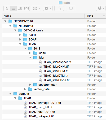
Download DatasetYou will want to create a data directory for all the Data Institute teaching
datasets. We suggest the pathway be ~/Documents/data/NEONDI-2016 or
the equivalent for your operating system. Once you've downloaded and unzipped
the dataset, move it to this directory.
Additional Resources
- R Markdown Cheatsheet: a very handy reference for using R Markdown
- R Markdown Reference Guide: a more expensive reference for R Markdown
- Introduction to R Markdown by Garrett Grolemund: a tutorial for learning R Markdown
Create an Rmd File
RMarkdown in RStudio Video
Our goal in this series is to document our workflow. We can do this by
- Creating an R Markdown (RMD) file in R studio and
- Rendering that RMD file to HTML using
knitr.
Watch this 6:38 minute video below to learn more about how you can convert an R Markdown
file to HTML (or other formats) using knitr in RStudio.
The text size in the video is small so you may want to watch the video in
full screen mode.
Now that you have a sense of how R Markdown can be used in RStudio, you are ready to create your own RMD document. Do the following:
- Create a new R Markdown file and choose HTML as the desired output format.
- Enter a Title (Explore NEON LiDAR Data) and Author Name (your name). Then click OK.
- Save the file using the following format: LastName-institute-week3.rmd NOTE: The document title is not the same as the file name.
- Hit the knit button in RStudio (as is done in the video above). What happens?
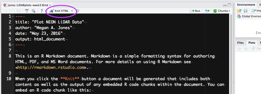
If everything went well, you should have an HTML format (web page) output after you hit the knit button. Note that this HTML output is built from a combination of code and documentation that was written using markdown syntax.
Next, we'll break down the structure of an R Markdown file.
Understand Structure of an R Markdown file
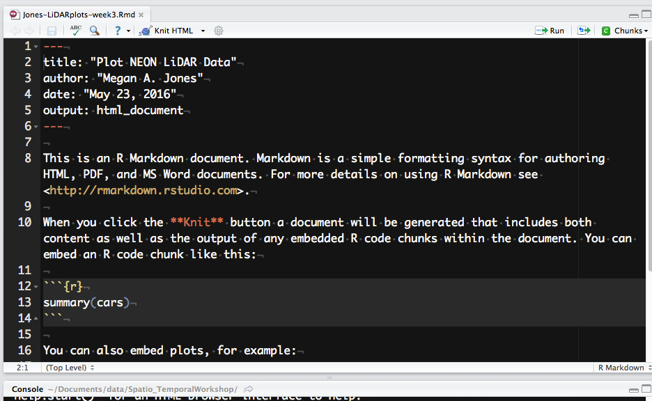
Let's next review the structure of an R Markdown (.Rmd) file. There are three
main content types:
- Header: the text at the top of the document, written in YAML format.
- Markdown sections: text that describes your workflow written using markdown syntax.
- Code chunks: Chunks of R code that can be run and also can be rendered using knitr to an output document.
Next let's explore each section type.
Header -- YAML block
An R Markdown file always starts with header written using YAML syntax. There are four default elements in the RStudio generated YAML header:
- title: the title of your document. Note, this is not the same as the file name.
- author: who wrote the document.
- date: by default this is the date that the file is created.
- output: what format will the output be in. We will use HTML.
A YAML header may be structured differently depending upon how your are using it. Learn more on the R Markdown documentation page.
- Title: Provide a title that fits the code that will be in your RMD.
- Author: Add your name here.
-
Output: Leave the default output setting:
html_document. We will be rendering an HTML file.
R Markdown Text/Markdown Blocks
An RMD document contains a mixture of code chunks and markdown blocks where you can describe aspects of your processing workflow. The markdown blocks use the same markdown syntax that we learned last week in week 2 materials. In these blocks you might describe the data that you are using, how it's being processed and and what the outputs are. You may even add some information that interprets the outputs.
When you render your document to HTML, this markdown will appear as text on the output HTML document.
Learn More about RStudio Markdown Basics
Explore Your R Markdown File
Look closely at the pre-populated markdown and R code chunks in your RMD file.
Does any of the markdown syntax look familiar?
- Are any words in bold?
- Are any words in italics?
- Are any words highlighted as code?
If you are unsure, the answers are at the bottom of this page.
- Remove the template markdown and code chunks added to the RMD file by RStudio. (Be sure to keep the YAML header!)
- At the very top of your RMD document - after the YAML header, add the bio and short research description that you wrote last week in markdown syntax to the RMD file.
- Between your profile and the research descriptions, add a header that says About My Project (or something similar).
- Add a new header stating R Markdown Activity and text below that explaining that this page demonstrates using some of the NEON Teakettle LiDAR data products in R. The wording of this text should clearly describe the code and outputs that you will be adding the page.
Code chunks
Code chunks are where your R code goes. All code chunks start and end with
``` – three backticks or graves. On
your keyboard, the backticks can be found on the same key as the tilde.
Graves are not the same as an apostrophe!
The initial line of a code chunk must appear as:
 ```{r chunk-name-with-no-spaces}
# code goes here
 ```
The r part of the chunk header identifies this chunk as an R code chunk and is
mandatory. Next to the {r, there is a chunk name. This name is not required
for basic knitting however, it is good practice to give each chunk a unique
name as it is required for more advanced knitting approaches.
Activity: Add Code Chunks to Your R Markdown File
Continue working on your document. Below the last section that you've just added, create a code chunk that loads the packages required to work with raster data in R.
```{r setup-library }

   library(rgdal)
   library(raster)

 ```
In R scripts, setting the working directory is normally done once near the beginning of your script. In R Markdown files, knit code chunks behave a little differently, and a warning appears upon kitting a chunk that sets a working directory.
```{r code-setwd}

   # set working directory to ensure R can find the file we wish to import.
   # This will depend on your local environment.
   setwd("~/Documents/data/NEONDI-2016/")

```
You changed the working directory to ~/Documents/data/NEONDI-2016/ (probably via setwd()). It will be restored to [directory path of current .rmd file]. See the Note section in ?knitr::knit ?knitr::knitThat's a bad sign if you want to set the working directory in one code chunk, and read or write data in another code chunk. To allow for a working data directory that is different from your Rmd file's current directory, you can store the directory path in a string variable.
```{r code-setwd-stringvariable}

	# set working directory as a string variable for use in other code chunks.
	# This will depend on your local environment.
	wd <- "~/Documents/data/NEONDI-2016/"
	setwd(wd)

 ```
The setwd(wd) line could be at the start of a lengthier code chunk that reads
from and writes to data files. Alternatively, since the variable will be kept in
this document's R environment, it can be used with paste() or paste0() when you
need to refer to a filepath. Proceed to the next step for an example of this.
(For further instruction on setting the working directory, see the NEON Data Skills tutorial Set A Working Directory in R.)
Let's add another chunk that loads the TEAK_lidarDSM raster file.
```{r load-dsm-raster }
   # check for the working directory
   getwd()
   # In this new chunk, the working directory has reverted to default upon kitting.
   # Combining the working directory string variable and
   # additional path to the file, import a DSM file.
   teak_dsm <- raster(paste0(wd, "NEONdata/D17-California/TEAK/2013/lidar/TEAK_lidarDSM.tif"))

 ```
Now run the code in this chunk.
You can run code chunks:
- Line-by-line: with cursor on current line, Ctrl + Enter (Windows/Linux) or Command + Enter (Mac OS X).
- By chunk: You can run the entire chunk (or multiple chunks) by clicking on the "Run" button in the upper right corner of the RStudio script panel and choosing the appropriate option (Run Current Chunk, Run Next Chunk). Keyboard shortcuts are available for these options.
Code chunk options
You can also add arguments or options to each code chunk. These arguments allow you to customize how or if you want code to be processed or appear on the output HTML document. Code chunk arguments are added on the first line of a code chunk after the name, within the curly brackets.
The example below, is a code chunk that will not be "run", or evaluated, by R. The code within the chunk will appear on the output document, however there will be no outputs from the code.
```{r intro-option, eval=FALSE}
# the code here will not be processed by R
# but it will appear on your output document
1+2
 ```
We use eval=FALSE often when the chunk is exporting an file that we don't
need to re-export but we want to document the code used to export the file.
Three common code chunk options are:
-
eval = FALSE: Do not evaluate (or run) this code chunk when knitting the RMD document. The code in this chunk will still render in our knitted HTML output, however it will not be evaluated or run by R. -
echo = FALSE: Hide the code in the output. The code is evaluated when the RMD file is knit, however only the output is rendered on the output document. -
results = hide: The code chunk will be evaluated but the results of the code will not be rendered on the output document. This is useful if you are viewing the structure of a large object (e.g. outputs of a largedata.frame).
Multiple code chunk options can be used for the same chunk. For more on code chunk options, read R Markdown: The Definitive Guide or the knitr documentation.
Update your RMD file as follows:
- Add a new code chunk that plots the
TEAK_lidarDSMraster object that you imported above. Experiment with plot colors and be sure to add a plot title. - Run the code chunk that you just added to your RMD document in R (e.g. run in console, not knitting). Does it create a plot with a title?
- In another new code chunk, import and plot another raster file from the NEON data subset
that you downloaded. The
TEAK_lidarCHMis a good raster to plot. - Finally, create histograms for both rasters that you've imported into R.
- Be sure to document your steps as you go using both code comments and markdown syntax in between the code chunks.
For help opening and plotting raster data in R, see the NEON Data Skills tutorial Plot Raster Data in R.
We will knit this document to HTML in the next tutorial.
Now continue on to the next tutorial to learn how to knit this document into a HTML file.
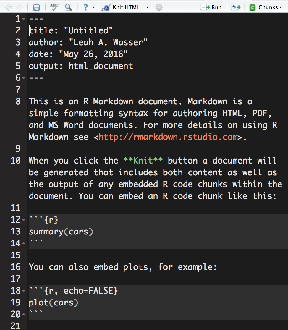
- Are any words in bold? - Yes, “Knit” on line 10
- Are any words in italics? - No
- Are any words highlighted as code? - Yes, “echo = FALSE” on line 22
Publish Code - From R Markdown to HTML with knitr
Last Updated: Apr 8, 2021
In this tutorial, we will cover the R knitr package that is used to convert
R Markdown into a rendered document (HTML, PDF, etc).
Learning Objectives
At the end of this activity, you will:
- Be able to produce (‘knit’) an HTML file from a R Markdown file.
- Know how to modify chunk options to change the output in your HTML file.
Things You’ll Need To Complete This Tutorial
You will need the most current version of R and, preferably, RStudio loaded on your computer to complete this tutorial.
Install R Packages
-
knitr:
install.packages("knitr") -
rmarkdown:
install.packages("rmarkdown")
Share & Publish Results Directly from Your Code!
The knitr package allow us to:
- Publish & share preliminary results with collaborators.
- Create professional reports that document our workflow and results directly from our code, reducing the risk of accidental copy and paste or transcription errors.
- Document our workflow to facilitate reproducibility.
- Efficiently change code outputs (figures, files) given changes in the data, methods, etc.
Publish from Rmd files with knitr
To complete this tutorial you need:
- The R
knitrpackage to complete this tutorial. If you need help installing packages, visit the R packages tutorial. - An R Markdown document that contains a YAML header, code chunks and markdown segments. If you don't have an .Rmd file, visit the R Markdown tutorial to create one.
How to Knit

To knit in RStudio, click the knit pull down button. You want to use the
knit HTML for this lesson.
When you click the Knit HTML button, a window will open in your console titled R Markdown. This pane shows the knitting progress. The output (HTML in this case) file will automatically be saved in the current working directory. If there is an error in the code, an error message will appear with a line number in the R Console to help you diagnose the problem.
Activity: Knit Script
Knit the .Rmd file that you built in the last tutorial. What does it look like?
View the Output
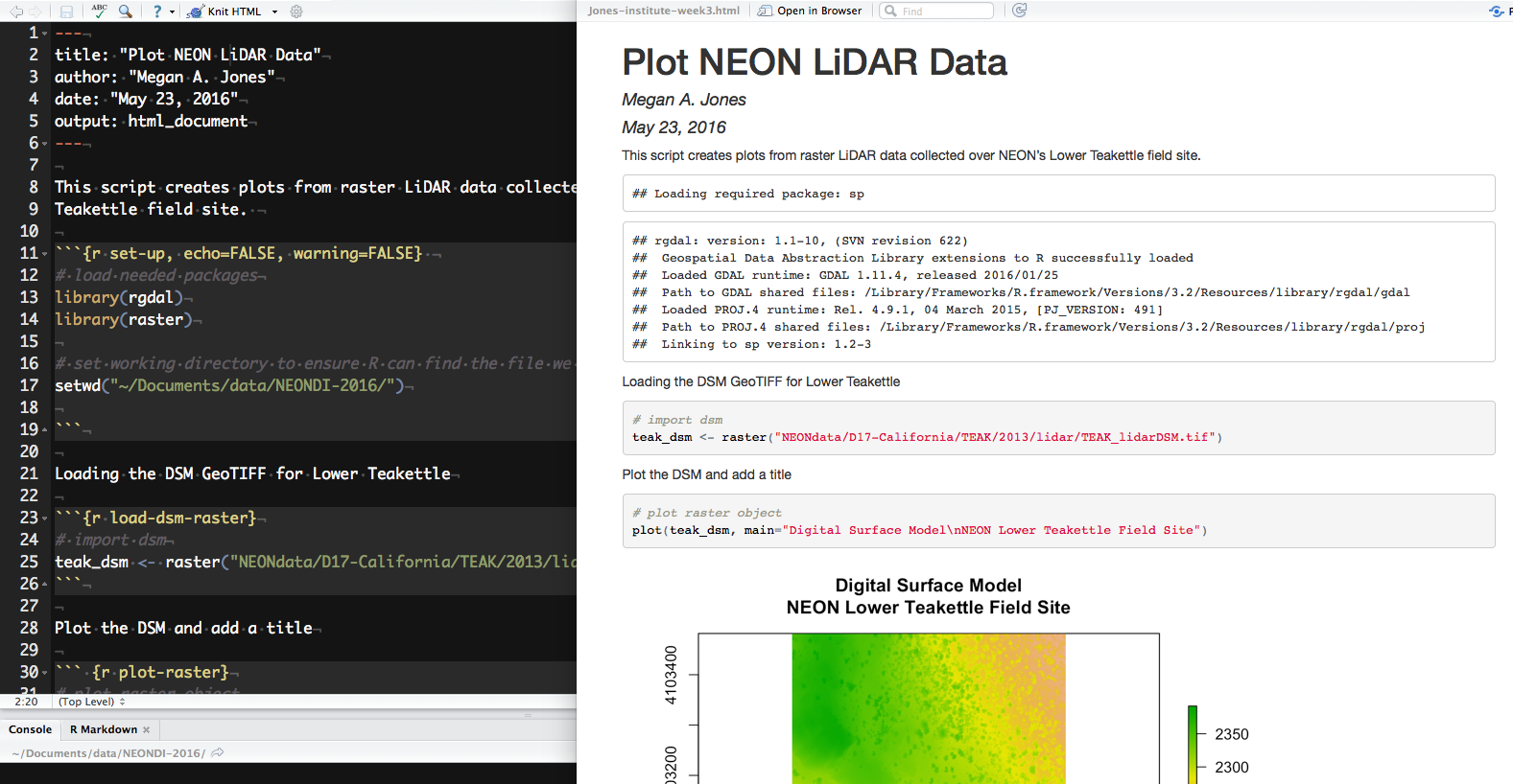
When knitting is complete, the new HTML file produced will automatically open.
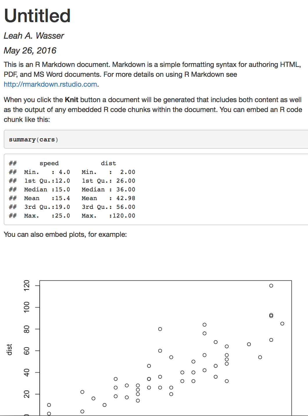
Notice that information from the YAML header (title, author, date) is printed at the top of the HTML document. Then the HTML shows the text, code, and results of the code that you included in the RMD document.
Data Institute Participants: Complete Week 2 Assignment
- Read this week’s assignment closely.
- Be sure to carefully check your knitr output to make sure it is rendering the way you think it should!
- When you are complete, submit your .Rmd and .html files to the NEON Institute participants GitHub repository (NEONScience/DI-NEON-participants).
- The files will have automatically saved to your R working directory, you will need to transfer the files to the /participants/pre-institute3-rmd/ directory and submitted via a pull request.