Explore Field Spectra Data - Scaling Ground and Airborne Observations

In this tutorial, we will demonstrate a scaling exercise to link the NEON field spectral reflectance and airborne spectrometer orthorectified surface directional reflectance datasets. We will also tie in the plant foliar traits data, which contains the geographic information and other metadata about the plants associated with the field spectra data.

Field spectral reflectance provide information about individual leaves or foliage, and samples such as these are often used as spectral end-members in classification applications. These data are measured with a hand-held Analytical Spectral Device (ASD). A collection of these spectral data can comprise a spectral library, eg. the USGS Spectral Library. This data product is collected on an opportunistic basis, typically in conjunction with NEON Airborne Observation Platform (AOP) overflights and in coordination with Terrestrial Observation System (TOS) Canopy Foliage Sampling. AOP typically collects spectra at 1-2 sites per year, so it is currently available at a subset of the NEON sites. The tutorial also demonstrates how to programmatically determine which data are available.

First, load the required libraries.

library(neonUtilities)

library(neonOS)

library(geoNEON)

library(ggplot2)

library(dplyr)

library(reshape2)

library(rhdf5)

library(terra)

Before downloading the data, we can explore the data product using the neonUtilities::getProductInfo. Let's take a look at the field spectra data product as follows. You can take a look at various components of the field_spectra_info variable as well by un-commenting the lines starting with View.

field_spectra_info <- neonUtilities::getProductInfo('DP1.30012.001')

#View(field_spectra_info$siteCodes) 

#View(field_spectra_info$siteCodes$availableDataUrls) # list available data urls

field_spectra_info$siteCodes$siteCode # list all available sites

##  [1] "DSNY" "GRSM" "GUAN" "HEAL" "ORNL" "OSBS" "PUUM" "RMNP" "SERC" "STEI" "TREE" "UNDE" "WREF" "YELL"

We can see that there are data available at 14 sites, as of the end of 2023.

Now that we know what sites have this field spectral data, let's take a look at one of the sites as an example - Rocky Mountain National Park (RMNP) in Colorado. We'll use this site to demonstrate some exploratory analysis you might start with when working with the field spectral data. To load this data directly into R, you can use the neonUtilities::loadByProduct function, specifying the data product ID (dpID) and site. Since this product is collected fairly infrequently, to date there is only one collection per year of this for the subset of sites shown above, so specifying the year-month in addition to the site is not necessary. This data is not too large in volume, so it should be fine to set the option check.size=FALSE. You will need to set package="expanded" in order to include the actual field spectral data.

field_spectra <- loadByProduct(dpID='DP1.30012.001',
                              site='RMNP',
                              package="expanded",
                              check.size=FALSE)

Let's take a look at all the associated tables contained in this data product, using the names function:

names(field_spectra)

## [1] "categoricalCodes_30012" "fsp_boutMetadata"       "fsp_sampleMetadata"     "fsp_spectralData"       "issueLog_30012"        
## [6] "per_sample"             "readme_30012"           "validation_30012"       "variables_30012"

We encourage looking at all of these tables to learn more about the data product, but you can find the actual data stored in the variables: fsp_boutMetadata (contains metadata information about this sampling bout), fsp_sampleMetadata (contains relevant metadata about the individual samples), fsp_spectralData (contains information about the individual sample data), and per_sample (contains the wavelength and reflectance data). Next, we can merge the fsp_spectralData, fsp_sampleMetadata and per_sample into a single data frame as follows. For more info on joining OS tables, please refer to https://www.neonscience.org/resources/learning-hub/tutorials/neonos-duplicates-joins.

list2env(field_spectra, .GlobalEnv)

spectra_data_metadata <- joinTableNEON(fsp_spectralData,fsp_sampleMetadata)

spectra_data <- merge(spectra_data_metadata,per_sample,by="spectralSampleID")

You can use View(spectra_data) to see the contents of this dataframe, or alternatively you could just print the variable name. The code below displays all the column names of this dataframe. We'll just show the head (or first 6 rows) of this data frame here, including a few of the columns.

colnames(spectra_data)

##  [1] "spectralSampleID"         "spectralSampleCode.x"     "locationID"               "uid.x"                    "domainID"                
##  [6] "siteID"                   "plotID"                   "plotType"                 "nlcdClass"                "geodeticDatum"           
## [11] "decimalLatitude"          "decimalLongitude"         "coordinateUncertainty"    "elevation"                "elevationUncertainty"    
## [16] "altLatitude"              "altLongitude"             "altCoordinateUncertainty" "collectDate.x"            "eventID"                 
## [21] "cfcIndividual"            "taxonID"                  "scientificName"           "sampleID"                 "sampleCode"              
## [26] "individualID"             "plantStatus"              "leafStatus"               "leafAge"                  "leafExposure"            
## [31] "leafSamplePosition"       "targetType"               "targetStatus"             "measurementVenue"         "measurementDate"         
## [36] "leafArrangement"          "remarks.x"                "collectedBy"              "recordedBy"               "dataQF.x"                
## [41] "publicationDate.x"        "release.x"                "uid.y"                    "software"                 "collectDate.y"           
## [46] "downloadFileUrl"          "downloadFileName"         "processedBy"              "reviewedBy"               "remarks.y"               
## [51] "dataQF.y"                 "publicationDate.y"        "release.y"                "spectralSampleCode.y"     "wavelength"              
## [56] "reflectanceCondition"     "reflectance"              "fileName"

head(spectra_data[c("spectralSampleID","taxonID","reflectance","wavelength","reflectanceCondition")],1)

##         spectralSampleID taxonID reflectance wavelength                        reflectanceCondition
## 1 FSP_RMNP_20200706_2043   POTR5 0.103038183        350 top of foliage (sunward) on white reference

You'll need to cast the wavelength and reflectance data to "numeric" data type, using as.numericin order to plot the data.

spectra_data$wavelength <- as.numeric(spectra_data$wavelength)

spectra_data$reflectance <- as.numeric(spectra_data$reflectance)

The spectral data is mainly composed of 3 columns: wavelength, reflectanceCondition, and reflectance. What is the reflectanceCondition? Let's look at the unique values represented:

unique(spectra_data$reflectanceCondition)

## [1] "top of foliage (sunward) on white reference"     "bottom of foliage (downward) on white reference"
## [3] "black reference"                                 "top of foliage (sunward) on black reference"    
## [5] "bottom of foliage (downward) on black reference"

This reflectanceCondition describes what exactly is being measured. As stated in the Field spectral data Quick Start Guide on the NEON Data Portal Field spectral data (DP1.30012.001) page, and explained in more detail in the NEON Field Spectra User Guide:

"Spectral reflectance of both the front and back of the sample is measured against a reflective white spectralon reference panel. A black spectralon reference is then measured, followed by spectral transmittance measurements of the front and back of the sample. Reference measurements of the white reference are taken between each leaf measurement."

first_spectra_plot <- ggplot(subset(spectra_data, spectralSampleID == "FSP_RMNP_20200706_2043"), 
                             aes(x =wavelength, y = reflectance,
                                 color = reflectanceCondition)) + geom_line() 

print(first_spectra_plot + ggtitle("FSP_RMNP_20200706_2043 spectra, all reflectance conditions"))

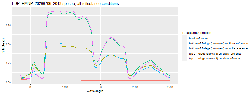
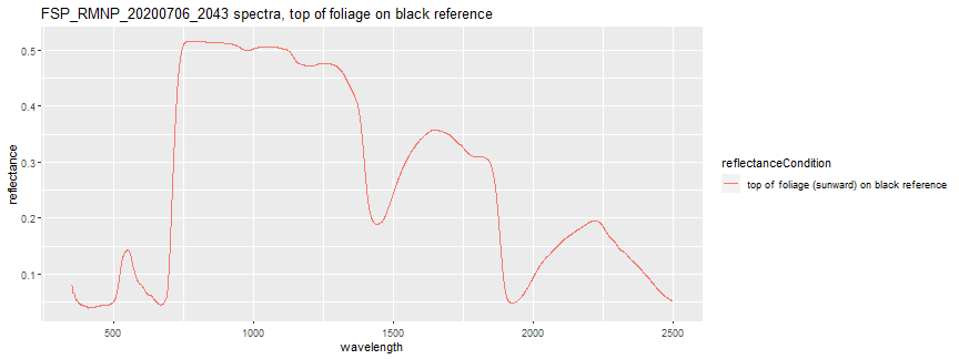
When linking with NEON's airborne spectral dataset (DP3.30006.001), the top of foliage (sunward) on black reference is the condition that we want to use. For this lesson, we will just focus on this reflectance condition. Let's take a look at the spectra for the single csv we read in.

To subset to plot only the top of foliage on black reference we can add 2nd condition:

first_spectra_plot <- ggplot(subset(spectra_data, spectralSampleID == "FSP_RMNP_20200706_2043" & reflectanceCondition == "top of foliage (sunward) on black reference"), aes(x =wavelength, y = reflectance, color = reflectanceCondition)) + geom_line() 

print(first_spectra_plot + ggtitle("FSP_RMNP_20200706_2043 spectra, top of foliage on black reference"))

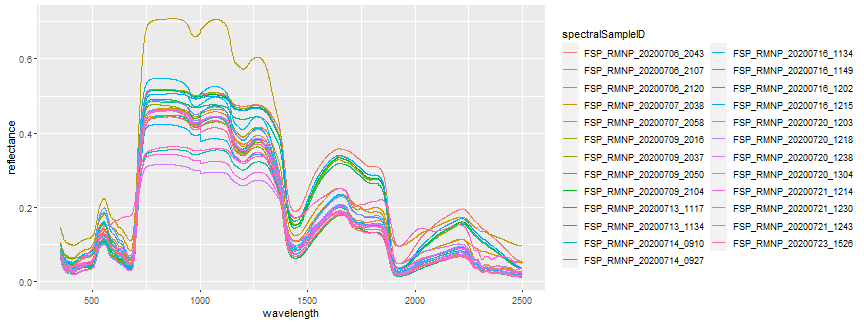
Next, let's plot the spectra of all the samples. First, let's extract only the reflectance condition we are interested in.

spectra_top_black <- spectra_data %>% dplyr::filter(reflectanceCondition == "top of foliage (sunward) on black reference")


ggplot(spectra_top_black, 
       aes(x =wavelength, y = reflectance,
           color = spectralSampleID)) + geom_line() 

Plot the spectra by taxon ID as follows:

ggplot(spectra_top_black, 
       aes(x =wavelength, y = reflectance,
           color = taxonID)) + geom_line(alpha = 0.5) 

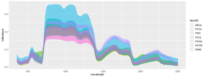
We can see there are 7 different species represented. We can get the count of each of the taxonIDs as follows. The filter(wavelength == 350) makes it so that we are not counting all 426 bands for each sample.

spectra_top_black %>% 
  filter(wavelength == 350) %>% 
  count(taxonID, sort = TRUE)

##   taxonID n
## 1   PICOL 5
## 2   PIPOS 5
## 3   POTR5 5
## 4    PIEN 3
## 5   PIFL2 3
## 6    PSME 3
## 7   ABLAL 1

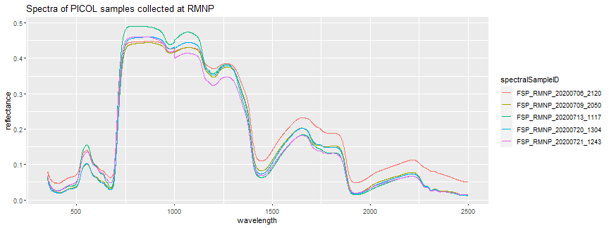
Let's dig in a a little more into the taxonIDs` which have multiple field spectra measurements. PICOL, PIPOS, and POTR5 each have 5 samples - these are the more common tree species at RMNP. Let's look at the spectra only from PICOL to start. For more details on this species, you can refer to the USDA PICOL plant profile page - we can see here that the common name of this species is "Lodgepole Pine".

picol_spectra_plot <- ggplot(subset(spectra_top_black, taxonID == "PICOL"), 
                             aes(x =wavelength, y = reflectance,
                                 color = spectralSampleID)) + geom_line() 

print(picol_spectra_plot + ggtitle("Spectra of PICOL samples collected at RMNP"))

What do you notice about these spectra? It looks like there is some variation between some of the samples, particularly in the visible portion of the spectrum. Let's go back to the original `spectra_merge` dataframe to see if we can determine more information about these individual samples. The code below pulls out some relevant columns from the data frame which may explain some of the variation we're seeing.

spectra_top_black[which(spectra_top_black$taxonID == "PICOL" & spectra_top_black$wavelength == 350), c("taxonID","spectralSampleID","plantStatus","leafStatus","leafAge","leafExposure","leafSamplePosition","targetType","targetStatus","measurementVenue","remarks.y")]

##       taxonID       spectralSampleID plantStatus leafStatus leafAge leafExposure leafSamplePosition   targetType targetStatus measurementVenue
## 4303    PICOL FSP_RMNP_20200706_2120          OK    healthy  mature     part-sun             middle pure foliage        fresh       laboratory
## 15058   PICOL FSP_RMNP_20200709_2050          OK    healthy  mature       sunlit                top pure foliage        fresh       laboratory
## 19360   PICOL FSP_RMNP_20200713_1117          OK    healthy  mature       sunlit             middle pure foliage        fresh       laboratory
## 43021   PICOL FSP_RMNP_20200720_1304          OK    healthy  mature       sunlit                top pure foliage        fresh       laboratory
## 49474   PICOL FSP_RMNP_20200721_1243          OK    healthy  mature       sunlit             middle pure foliage        fresh       laboratory
##                                              remarks.y
## 4303                           all parallel needle mat
## 15058            RMNP bristlecone pine long needle mat
## 19360           PICOL-2 horizontal needle mat sample 2
## 43021 cfc.RMNP005.PICOL2-1.20200720 tape on both sides
## 49474                     cfc.RMNP006.PICOL-1.20200721

Here, we can see that all the plants have an "OK" status, and all the leaves have a "healthy" status, but the leafExposure and leafSamplePosition vary between the samples. This may cause some variation in the spectral signature. Some variation is expected, even if all conditions are identical, as there is uncertainty associated with any measurement, due to the properties of the leaf being sample, and the measurements themselves.

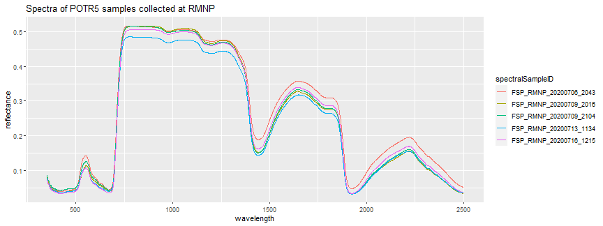
Let's also plot the spectra of one of the other more common Rocky Mountain species: POTR5 (Quaking Aspen), to explore some of the typical variation you might see in the spectral signatures of a single species.

potr5_spectra_plot <- ggplot(subset(spectra_top_black, taxonID == "POTR5"), 
                             aes(x =wavelength, y = reflectance,
                                 color = spectralSampleID)) + geom_line() 

print(potr5_spectra_plot + ggtitle("Spectra of POTR5 samples collected at RMNP"))

Finally, it may be useful to plot the spectra of two species on the same plot in order to compare the signatures. For this example, we'll show PICOL (Lodgepole Pine) and POTR5 (Quaking Aspen) together, including all 5 measurements of each.

potr5_picol_plot <- ggplot(subset(spectra_top_black, taxonID %in% c("POTR5","PICOL")), 
                             aes(x =wavelength, y = reflectance,
                                 color = taxonID)) + geom_line(alpha = 0.5) 

print(potr5_picol_plot + ggtitle("Comparison PICOL (Lodgepole Pine) and POTR5 (Aspen) Leaf sample spectra at RMNP"))

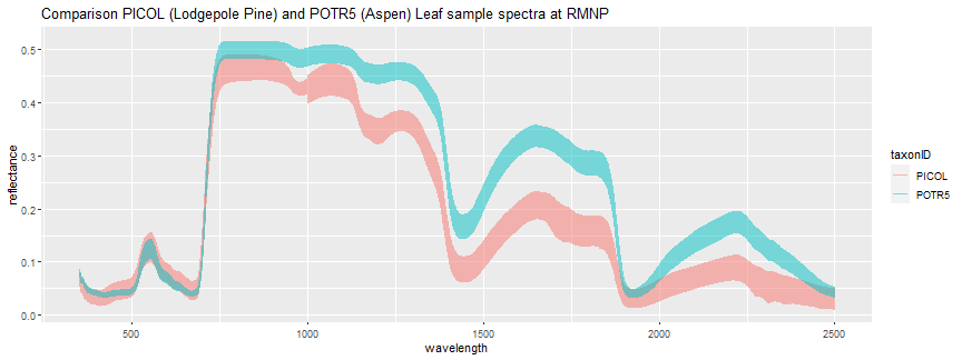
Here we can see that while there is considerable overlap in the visible portion of the electromagnetic spectrum, there are some distinct differences in the spectral signatures between these two species, particularly in the near to shortwave infrared regions.

Foliar Trait Data

As described in the Field Spectra Data Quick Start Guide,

"To find the geographic location of each plant, use the plant crown shapefiles in the Plant foliar physical and chemical properties data product (DP1.10026.001, table cfc_shapefile). For the locations of plants that have not been mapped to shapefiles, follow the instructions in the Data Product User Guide for DP1.10026.001."

This next section outlines how you would go about finding the geolocation information for the field spectra data. This is necessary if you are linking with the AOP hyperspectral data, which we will demonstrate next. We will start by demonstrating how to pull in the spectra of the single pixel. Not all foliar data have crown polygons, so this method is useful if the crown polygon data is not available. We will also demonstrate how to pull in the crown polygon shapefiles, and use that to extract the reflectance, at the end. This method requires a few extra steps.

Let's start by looking at the product information for this foliar trait data product. As before, you can un-comment the #View lines to explore this dataset more.

foliar_trait_info <- neonUtilities::getProductInfo('DP1.10026.001')

#View(foliar_trait_info$siteCodes)

#View(foliar_trait_info$siteCodes$availableDataUrls)

We can get the availableDataUrls of the RMNP site as follows. This step is not required, but as we showed with the field spectral data, this is a way to see what foliar trait data are available for a given site, since the canopy foliar sampling does not occur every year.

# view the RMNP foliar trait available data urls

foliar_trait_info$siteCodes[which(foliar_trait_info$siteCodes$siteCode == 'RMNP'),c("availableDataUrls")]

## [[1]]
## [1] "https://data.neonscience.org/api/v0/data/DP1.10026.001/RMNP/2020-07"

Let's download the foliar trait data from 2020-07 at RMNP to obtain the precise locations of the foliar spectra samples.

foliar_traits <- loadByProduct(dpID='DP1.10026.001',
                               site='RMNP',
                               startdate='2020-07',
                               package="expanded",
                               check.size=FALSE)

names(foliar_traits)

We can use the geoNEON package to obtain the refined geolocation information, based on product-specific rules and spatial designs. For more details on this package, please refer to the Access and Work with NEON Geolocation Data tutorial.

vst.loc <- getLocTOS(data=foliar_traits$vst_mappingandtagging,
                     dataProd="vst_mappingandtagging")

Now let's merge the foliar traits cfc_fieldData with this vst.loc data, which now includes the refined (adjusted) locations.

foliar_traits_loc <- merge(foliar_traits$cfc_fieldData,vst.loc,by="individualID")

Finally, we can merge this foliar_traits_loc data frame with the spectra_merge data frame by the sampleID in order to link the field spectra samples with the geolocation information. Note that there is also a crownPolygonID column, which contains the id of the crown polygon shape file. We will hold off on using this crown polygon for now, but will start by using the adjusted geolocations calculated using geoNEON to obtain the corresponding airborne reflectance data.

Since the spectra_top_black table includes the wavelength and reflectance values for all 426 bands, we can first subset it to only include a single wavelength.

spectra_traits <- merge(spectra_top_black,foliar_traits_loc,by="sampleID")

# display values of only first wavelength for each sample

spectra_traits_sub <- merge(spectra_top_black[spectra_top_black$wavelength == 350,],foliar_traits_loc,by="sampleID")

spectra_traits_sub[c("spectralSampleID","taxonID","stemDistance","stemAzimuth","adjEasting","adjNorthing","crownPolygonID")]

##          spectralSampleID taxonID stemDistance stemAzimuth adjEasting adjNorthing  crownPolygonID
## 1  FSP_RMNP_20200716_1215   POTR5         10.4        28.3   459058.0     4450439 RMNP.03861.2020
## 2  FSP_RMNP_20200714_0910   PIFL2          5.8       143.5   458176.5     4449625 RMNP.04352.2020
## 3  FSP_RMNP_20200716_1149   PIFL2         16.9        14.0   459046.8     4450436 RMNP.03832.2020
## 4  FSP_RMNP_20200709_2050   PICOL         17.6       278.2   453521.1     4458506 RMNP.02496.2020
## 5  FSP_RMNP_20200706_2120   PICOL          5.8        83.0   453949.4     4448624 RMNP.03472.2020
## 6  FSP_RMNP_20200709_2104   POTR5         15.0       335.8   453532.4     4458517 RMNP.02510.2020
## 7  FSP_RMNP_20200709_2037    PIEN         11.2       325.1   453558.6     4458691 RMNP.02898.2020
## 8  FSP_RMNP_20200720_1238    PSME          9.6       141.1   455181.1     4446533 RMNP.04033.2020
## 9  FSP_RMNP_20200713_1134   POTR5          2.0        50.0   460123.7     4449762 RMNP.03623.2020
## 10 FSP_RMNP_20200709_2016   POTR5         12.1       347.1   453582.6     4458674 RMNP.02875.2020
## 11 FSP_RMNP_20200721_1230    PIEN          8.5       129.3   453707.2     4445454 RMNP.05230.2020
## 12 FSP_RMNP_20200723_1526   PIPOS         22.2       328.2   459502.2     4445010 RMNP.03698.2020
## 13 FSP_RMNP_20200716_1134   PIPOS         11.1        51.5   459051.4     4450427 RMNP.03823.2020
## 14 FSP_RMNP_20200706_2043   POTR5          6.7        93.2   453949.4     4448643 RMNP.03511.2020
## 15 FSP_RMNP_20200721_1243   PICOL          3.6       235.9   453718.4     4445458 RMNP.05247.2020
## 16 FSP_RMNP_20200714_0927   PIPOS         15.8       326.9   458184.2     4449622 RMNP.04348.2020
## 17 FSP_RMNP_20200720_1304   PICOL          9.2        49.7   455181.6     4446526 RMNP.04015.2020
## 18 FSP_RMNP_20200706_2107    PIEN          7.6       140.0   453947.6     4448637 RMNP.03507.2020
## 19 FSP_RMNP_20200720_1203   PIFL2          6.0       329.1   455190.8     4446525 RMNP.04021.2020
## 20 FSP_RMNP_20200707_2038    PSME         18.8       268.5   456373.2     4450501 RMNP.03880.2020
## 21 FSP_RMNP_20200721_1214   ABLAL          6.4       299.6   453715.4     4445443 RMNP.04893.2020
## 22 FSP_RMNP_20200720_1218   PIPOS          7.5       299.0   455187.3     4446524 RMNP.04022.2020
## 23 FSP_RMNP_20200707_2058   PIPOS          7.4        73.0   456379.8     4450485 RMNP.03868.2020
## 24 FSP_RMNP_20200716_1202    PSME         16.4       338.2   459056.9     4450435 RMNP.03836.2020
## 25 FSP_RMNP_20200713_1117   PICOL          9.3        25.4   460126.2     4449769 RMNP.03626.2020

Great, now we have the field spectra data and the corresponding locations of the leaf-clip samples.

Airborne Reflectance Data

For the final part of this lesson, we will download the airborne reflectance data, and use some R functions to read the reflectance data into a terra:rast Spatial Object, and extract the spectral signature of the pixel corresponding to the location of the leaf-clip sample. We can use the neonUtilities::byTileAOP function to download only the 1km x 1km tile that contains the data we're interested in. First, let's set the working directory to where we want to download the data.

# set working directory (this will depend on your local environment)

wd <- "~/data/"

setwd(wd)

We will download the corresponding reflectance spectra of the pixel corresponding to where a single PICOL sample was located. Let's extract that sample from the spectral_traits table so we can easily pull out the geographic information.

fsp_rmnp_picol_20200720_1304 <- spectra_traits[spectra_traits$spectralSampleID == "FSP_RMNP_20200720_1304",]

Download the reflectance data that encompasses this data point. Reflectance data can be quite large (~500-600+ MB per tile), so for this example, we'll only download the single tile needed. We'll leave the check.size field empty (default is TRUE), which means you will need to enter y in order to continue the download.

byTileAOP(dpID='DP3.30006.001',

          site='RMNP',

          year=2020,

          easting=fsp_rmnp_picol_20200720_1304$adjEasting,

          northing=fsp_rmnp_picol_20200720_1304$adjNorthing,

          savepath=wd)

This file will be downloaded into a nested subdirectory under the ~/data folder, inside a folder named DP3.30006.001 (the Data Product ID of the aerial reflectance data). The file should show up in this location: ~/data/DP3.30006.001/neon-aop-products/2020/FullSite/D10/2020_RMNP_3/L3/Spectrometer/Reflectance/NEON_D10_RMNP_DP3_455000_4446000_reflectance.h5. Let's define an h5_file variable that points to the full path to this file.

# Define the h5 file name to be opened

h5_file <- paste0(wd,"DP3.30006.001/neon-aop-products/2020/FullSite/D10/2020_RMNP_3/L3/Spectrometer/Reflectance/NEON_D10_RMNP_DP3_455000_4446000_reflectance.h5")

Now we can use some pre-defined functions for working with the airborne reflectance data. For more details, please refer to the Introduction to Hyperspectral Remote Sensing tutorial series.

geth5metadata <- function(h5_file){
  # get the site name
  site <- h5ls(h5_file)$group[2]
  
  # get the wavelengths
  wavelengths <- h5read(h5_file,paste0(site,"/Reflectance/Metadata/Spectral_Data/Wavelength"))
  
  # get the epsg code
  h5_epsg <- h5read(h5_file,paste0(site,"/Reflectance/Metadata/Coordinate_System/EPSG Code"))
                    
  # get the Reflectance_Data attributes
  refl_attrs <- h5readAttributes(h5_file,paste0(site,"/Reflectance/Reflectance_Data"))
  
  # grab the UTM coordinates of the spatial extent
  xMin <- refl_attrs$Spatial_Extent_meters[1]
  xMax <- refl_attrs$Spatial_Extent_meters[2]
  yMin <- refl_attrs$Spatial_Extent_meters[3]
  yMax <- refl_attrs$Spatial_Extent_meters[4]
  
  ext <- ext(xMin,xMax,yMin,yMax) # define the extent (left, right, top, bottom)

  no_data <- as.integer(refl_attrs$Data_Ignore_Value)  # define the no data value
  meta_list <- list("wavelengths" = wavelengths, "crs" = crs(paste0("epsg:",h5_epsg)), "raster_ext" = ext, "no_data_value" = no_data)
  h5closeAll() # close all open h5 instances
  
  return(meta_list)
}

  band2Raster <- function(h5_file, band, extent, crs, no_data_value){
    site <- h5ls(h5_file)$group[2] # extract the site info
    # read in the raster for the band specified, this will be an array
    refl_array <- h5read(h5_file,paste0(site,"/Reflectance/Reflectance_Data"),index=list(band,NULL,NULL))
	  refl_matrix <- (refl_array[1,,]) # convert from array to matrix
	  refl_matrix <- t(refl_matrix) # transpose data to fix flipped row and column order
    refl_matrix[refl_matrix == no_data_value] <- NA     # assign data ignore values to NA
    refl_out <- rast(refl_matrix,crs=crs) # write out as a raster
    ext(refl_out) <- extent # assign the extents to the raster
    h5closeAll() # close all open h5 instances
    return(refl_out) # return the terra raster object
}

Now that we've defined these functions, we can run lapply on the band2Raster function, using all the bands. This may take a minute or two to complete.

# get the relevant metadata using the geth5metadata function

h5_meta <- geth5metadata(h5_file)

# get all bands - a consecutive list of integers from 1:426 (# of bands)

all_bands <- as.list(1:length(h5_meta$wavelengths))

# lapply applies the function `band2Raster` to each element in the list `all_bands`

refl_list <- lapply(all_bands,
                    FUN = band2Raster,
                    h5_file = h5_file,
                    extent = h5_meta$raster_ext,
                    crs = h5_meta$crs,
                    no_data_value = h5_meta$no_data_value)

refl_rast <- rast(refl_list)

We can also plot an RGB image. First we'll run lapply on the band2Raster function, this time using a list only consisting of the RGB bands:

rgb <- list(58,34,19)

# lapply applies the function to each element in the RGB list

rgb_list <- lapply(rgb,
                    FUN = band2Raster,
                    h5_file = h5_file,
                    extent = h5_meta$raster_ext,
                    crs = h5_meta$crs,
                    no_data_value = h5_meta$no_data_value)

rgb_rast <- rast(rgb_list)

Let's plot the RGB image of the reflectance tile, for reference. We will also include the location of the tree that the leaf clip data were sampled from (tree_loc).

plotRGB(rgb_rast,stretch='lin',axes=TRUE)

#convert the data frame into a shape file (vector)

tree_loc <- vect(cbind(fsp_rmnp_picol_20200720_1304$adjEasting,
                       fsp_rmnp_picol_20200720_1304$adjNorthing), crs=h5_meta$crs)

plot(tree_loc, col="red", add = T)

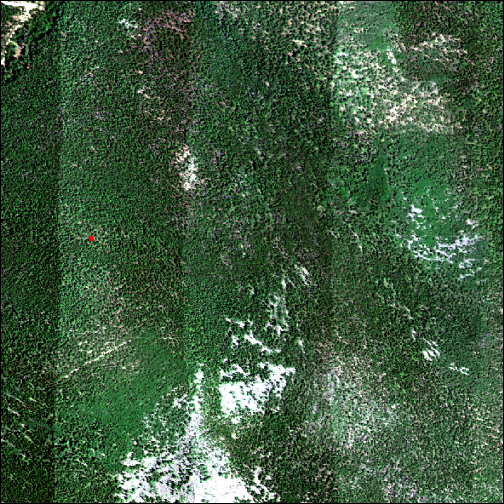
It's a little easier to see the sample location if we zoom in on a smaller area.

x_sub = c(455150, 455200)

y_sub = c(4446500, 4446550)

plotRGB(rgb_rast,stretch='lin',xlim=x_sub,ylim=y_sub)

plot(tree_loc, col="red", add = T)

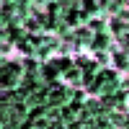
Next we can extract the aerial reflectance spectra using the terra::extract function as follows. We'll create a data frame of the wavelengths and reflectance of that pixel so we can plot using ggplot.

refl_air <- extract(refl_rast, 
                    cbind(fsp_rmnp_picol_20200720_1304$adjEasting[1],
                          fsp_rmnp_picol_20200720_1304$adjNorthing[1]))

refl_air_df <- data.frame(t(refl_air))

refl_air_df$wavelengths <- h5_meta$wavelengths

names(refl_air_df) <- c('reflectance','wavelength')

refl_air_df$reflectance <- refl_air_df$reflectance/10000 #scale by reflectance scale factor (10,000)

picol_air_plot <- ggplot(refl_air_df, aes(x=wavelength, y=reflectance)) + geom_line() + ylim(0,.25)

print(picol_air_plot + ggtitle("Airborne Reflectance Spectra of PICOL at RMNP"))

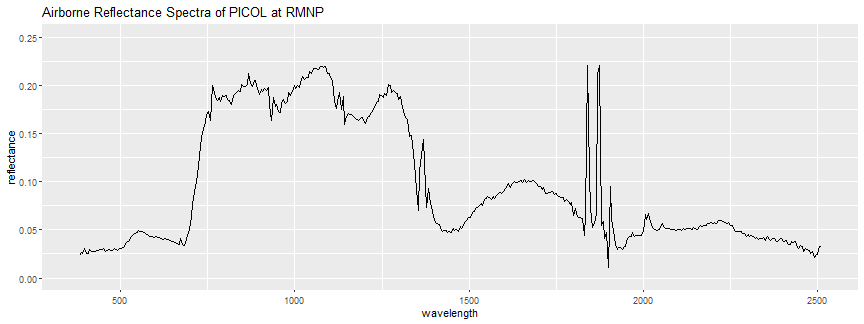
The shape of the spectra looks similar to the leaf-clip spectra, however you might notice some key differences. This spectral curve is not quite as smooth as the leaf-clip spectra - this is partly because of additional noise (uncertainty) introduced due to the nature of the remotely-sensed data. The airborne reflectance is collected at ~1000 m above the ground, and each pixel represents a 1 m x 1 m area (instead of just a single leaf). The airborne hyperspectral sensor is recording not only what's on the ground, but also the atmosphere between the airplane and the ground. While an atmospheric correction is applied (as well as other corrections) to generate the surface directional reflectance, additional uncertainty is introduced. Also, note that there are some regions around the ~1400 nm and ~1800 nm wavelengths with some large anomalous values. These are the water-vapor absorption bands, regions where gasses in the atmosphere (primarily carbon dioxide and water vapor) absorb radiation, and obscure the reflected radiation that the imaging spectrometer measures. For more detailed information about the absorption bands, and airborne reflectance data, please refer to the Introduction to Hyperspectral Remote Sensing Data tutorial series.

Plotting Leaf-Clip and Airborne Data Together

Finally, let's make a plot of these two spectra (leaf-clip and aerial reflectance) together. First, make a combined dataframe, then plot with ggplot.

# create a combined dataframe of the leaf clip spectra (fsp_rmnp_picol) and the tree crown pixel spectra (picol_crown_df)

fsp_air_combined_df <- bind_rows(fsp_rmnp_picol_20200720_1304[c("wavelength","reflectance")],refl_air_df[c("wavelength","reflectance")])



# add a new column to indicate data source

fsp_air_combined_df$spectra_source <- c(rep("leaf-clip reflectance", nrow(fsp_rmnp_picol_20200720_1304)), rep("airborne reflectance", nrow(refl_air_df)))



spectra_plot <- ggplot() + 
  geom_line(data=fsp_air_combined_df, aes(x=wavelength, y=reflectance, color=spectra_source), show.legend=TRUE) +
  labs(x="Wavelength (nm)",  y="Reflectance") +
  theme(legend.position = c(0.8, 0.8)) +  ylim(0, 0.5)



print(spectra_plot + ggtitle("Spectra of PICOL Leaf Clip Sample & Corresponding Airborne Pixel at RMNP"))

Why is there a difference between the leaf-clip spectra and the remotely-sensed spectra of the corresponding pixel?

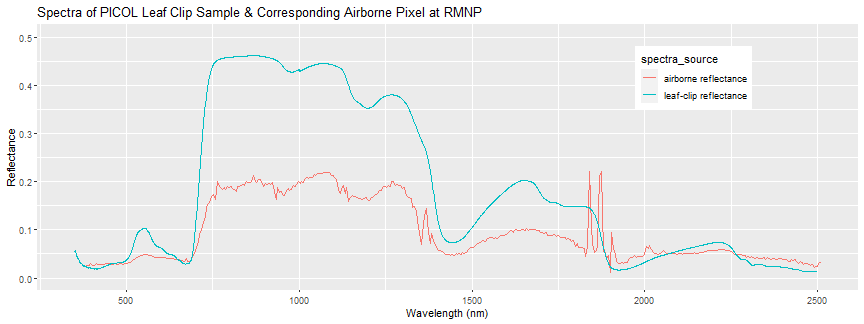
Each reflectance pixel represents a 1m x 1m area, so it contains an average spectra of all the vegetation and non-vegetation that are contained in that area. For example, a single pixel could contain the reflectance of a mix of leaves as well as branches, and any gaps in the tree canopy (eg. the ground under the tree). This averaging is called "spectral mixing" and you can perform "spectral un-mixing" to decompose an average spectra into it's component parts. These leaf clip spectra can be used as "end-members", in classification applications, for example.

Also, it is important to understand that there are uncertainties in the ASD measurements as well as the airborne spectra. There may be some geographic uncertainty associated with both the airborne data (which has 0.5 m horizontal resolution), as well as with the field sample geolocations. There is also some uncertainty in the spectral data itself. For example, there is uncertainty resulting from the atmospheric correction applied when generating the reflectance data from the at-sensor-radiance. Weather conditions during the flight are important to consider as well. The Airborne Observation Platform attempts to collect the coincident overflights in clear weather, but this may not always be the case. For more on hyperspectral uncertainties and variation, please refer to the Spectrometer Mosaic ATBD (Algorithm Theoretical Basis Document).

Incorporating Tree Crown Polygon Shapefiles

Starting in 2020 (including RMNP 2020), the foliar traits data products include shape files of the polygons of the tree crowns where the samples are taken from. The crown shapefiles are not available for all of the canopy foliar data, but if they are available, it is recommended to use them. The last part of the lesson demonstrates how to download the tree crown shape files, and plots the spectra of the airborne reflectance data of all the pixels inside the tree crown area.

First, we can use the neonUtilities::loadByProduct and zipsByURI functions to download all the tree crown polygon shapefile data, as follows. This is also the recommended way to determine which crown polygon data are available, across all the sites.

crown_polys <- loadByProduct(dpID='DP1.10026.001', 

                          tabl='cfc_shapefile', 

                          include.provisional=T,

                          check.size=F)

zipsByURI(crown_polys, savepath=paste0(wd,'crown_polygons'),check.size=FALSE)

Next we can read in the polygon data as a terra SpatVector object as follows. Display the coordinate reference system (CRS) information. You can un-comment the last line to display more detailed information about the CRS.

shp_file <- paste0('~/data/','RMNP/RMNP-2020-polygons-v2/RMNP-2020-polygons.shp')

rmnp_crown_poly <- terra::vect(shp_file)

crs(rmnp_crown_poly, describe=TRUE) # display dataframe describing the CRS

##                       name authority code                              area                         extent
## 1 WGS 84 / Pseudo-Mercator      EPSG 3857 World between 85.06°S and 85.06°N -180.00, 180.00, 85.06, -85.06

# cat(crs(rmnp_crown_poly), "\n")

You can see that this data has EPSG code 3857, which does not match the AOP raster data, which is in UTM 13N (EPSG 32613) for this site. We can re-project the vector data so that both datasets align. Note that NEON is planning to update the CRS of the polygon data to match the AOP raster data, but this is not currently available (as of Spring 2024).

rmnp_crown_poly_UTM13N <- project(rmnp_crown_poly, "EPSG:32613")

Let's plot the crown polygon data (orange line) along with the RGB reflectance image and tree location (red point).

plotRGB(rgb_rast,stretch='lin',xlim=x_sub,ylim=y_sub,axes=TRUE) # plot reflectance RGB raster data

plot(tree_loc, col="red", add = T) # plot the location of the tree (red point)

picol_crown_poly <- rmnp_crown_poly_UTM13N[rmnp_crown_poly_UTM13N$crownPolyg == "RMNP.04015.2020"]

plot(picol_crown_poly, border = "orange", lwd = 2, add=T) # plot the tree crown polygon

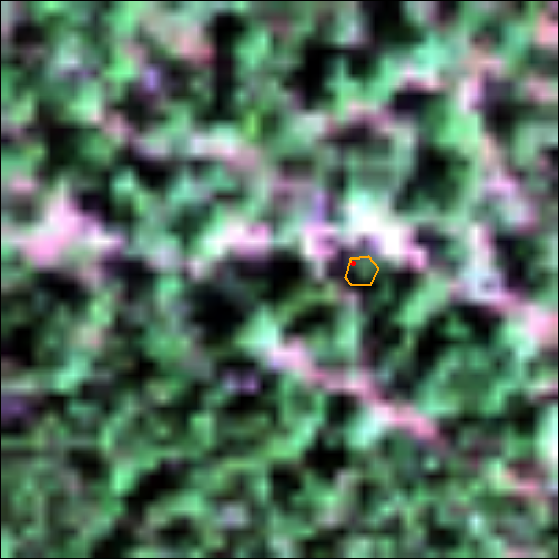
We can again use terra:extract to pull out the reflectance values of all the pixels inside this area. Then use the reshape2::melt function to reformat the data so it is simpler to plot.

refl_crown <- extract(refl_rast, picol_crown_poly,ID=FALSE)

refl_crown_df <- data.frame(t(refl_crown))

refl_crown_df$wavelengths <- h5_meta$wavelengths

names(refl_crown_df) <- c('1','2','3','4','5','6','wavelength')

row.names(refl_crown_df) <- NULL #reset the row names so they represent the band #s

picol_crown_df <- melt(refl_crown_df, id.vars = 'wavelength', value.name = 'reflectance', variable.name = 'crown_pixel')

# head(picol_crown_df[c("crown_pixel","wavelength","reflectance")]) #optionally display the first part of the data

Plot the spectra of all the pixels in the tree crown polygon, first applying the reflectance scale factor.

picol_crown_df$reflectance <- (picol_crown_df$reflectance/10000)

picol_crown_plot <- ggplot(picol_crown_df, aes(x=wavelength, y=reflectance, color=crown_pixel)) + 
  labs(x="Wavelength (nm)",  y="Reflectance") + geom_line() + ylim(0,0.35)

print(picol_crown_plot + ggtitle("Airborne Reflectance Spectra of Tree Crown Polygon Pixels of PICOL at RMNP"))

Great, we've plotted the reflectance curves of all the pixels captured within the tree crown polygon area. What might cause some of the differences between these spectral signatures? Lastly, let's plot the reflectance of the airborne hyperspectral data (all pixels in the tree-crown polygon) along with the ground-measured leaf-clip spectra.

# create a combined dataframe of the leaf clip spectra (fsp_rmnp_picol) and the tree crown pixel spectra (picol_crown_df)

combined_df <- bind_rows(fsp_rmnp_picol_20200720_1304[c("wavelength","reflectance")],picol_crown_df[c("wavelength","reflectance")])

# add a new column to indicate spectra data source

combined_df$spectra_source <- c(rep("leaf-clip reflectance", nrow(fsp_rmnp_picol_20200720_1304)), rep("airborne reflectance", nrow(picol_crown_df)))

spectra_crown_plot <- ggplot() + 
  geom_line(data=combined_df, aes(x=wavelength, y=reflectance, color=spectra_source), show.legend=TRUE) +
  labs(x="Wavelength (nm)",  y="Reflectance") + theme(legend.position = c(0.8, 0.8)) +  ylim(0, 0.5)

print(spectra_crown_plot + ggtitle("Spectra of PICOL Leaf Clip Sample & Corresponding Airborne Tree-Crown Pixels at RMNP"))

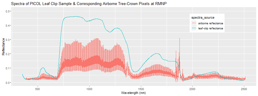
Again we can see there is some discrepancy between the airborne and field spectra, and there is a decent amount of variation between the spectra of the pixels contained within the tree crown polygon. The leaf-clip spectra is one "end-member" that contributes to the 1-m pixel combined reflectance. The exploratory analysis demonstrated in this tutorial is an example of some steps you might take to get a feel for the data. We recommend you explore some other samples at this site, or field spectra data at another site, building off this R code to answer some questions you come up with as you start digging into the data.