Series
Intro to AOP Data in Google Earth Engine (GEE) Tutorial Series
NEON has uploaded a subset of AOP data into Earth Engine in a public repository for scientists to work with remote sensing data in this geospatial cloud-computing platform. These data can be found on the GEE Publisher Datasets Page (https://developers.google.com/earth-engine/datasets/publisher/neon-prod-earthengine). The AOP image collections includes hyperspectral surface bidirectional reflectance, surface directional reflectance, discrete lidar derived rasters (i.e. digital elevation models - DEM and canopy height models - CHM), and RGB camera imagery at a subset of NEON sites spanning the United States, over multiple (1-5+) years at each site. To browse and interact with the available AOP data in a GEE app, click here: https://neon-prod-earthengine.projects.earthengine.app/view/neon-aop-gee-data-viewer---desktop. Additional datasets can be added upon request, using the NEON Contact Us form.
This Data Skills series walks new Google Earth Engine users through visualizing and working with NEON AOP datasets in GEE, including annotated Google Earth Engine scripts using the JavaScript API. The series starts with a basic lesson that introduces the Earth Engine Code Editor and explains how to read in the AOP Image Collections and explore relevant properties and metadata. The subsequent tutorials continue through some pre-processing workflows (eg. masking out bad-weather data) and onto more advanced visualization, exploration and analysis using AOP data in Earth Engine.
To follow along with this series, you will first need to register for an Earth Engine account, as described in the requirements at the beginning of the first lesson. Once you have an account, the GEE code for each lesson can be opened and run directly in the Earth Engine Code Editor by clicking the "Get Lesson Code" link at the bottom of each page. Click on the linked titles in the bar to the left to get started.
Introduction to AOP Public Datasets in Google Earth Engine (GEE)
Authors: Bridget Hass, John Musinsky
Last Updated: Mar 12, 2026
NEON AOP Data in Google Earth Engine
Google Earth Engine (GEE) is a free and powerful cloud-computing platform for carrying out remote sensing and geospatial data analysis. In this tutorial, we introduce you to the NEON AOP datasets that have been added to Google Earth Engine as Publisher Datasets.

NEON is planning to add the full archive of AOP L3 Surface Bidirectional Reflectance, LiDAR Elevation, Ecosystem Structure (CHM), High-resolution orthorectified camera imagery and Canopy nitrogen (a subset of data newly available as of Feb 2026). Since the L3 Surface Directional Reflectance is planned to be replaced by the bidirectional (Bidirectional Reflectance Distribution Function (BRDF) and topographic corrected) reflectance as that is processed and becomes available, we are only adding directional reflectance data to GEE upon request. As of March 2026, bidirectional data is only available for AOP data collected between 2022-2025, but re-processing of older AOP data (2013-2021) will begin in Spring 2026. Please see the tutorial Introduction to Bidirectional Hyperspectral Reflectance Data in Python for more information on the differences between the directional and bidirectional reflectance data products.
Not all of the data that is available on the NEON Data Portal is currently available in GEE, so this tutorial shows you how to find which data are currently available in GEE. If there are certain NEON sites and years of data you would like to see added to Google Earth Engine sooner, use the NEON Contact Us form to request this, and include "Google Earth Engine Remote Sensing Data" in the text.
Objectives
After completing this activity, you will become familiar with:
- Google Earth Engine (GEE)
- NEON AOP Image Collections in GEE
And you will be able to:
- Write and run basic JavaScript code in the GEE Code Editor
- Discover which NEON AOP datasets are available in GEE
- Explore the NEON AOP GEE Image Collections
- Plot an RGB image of a reflectance dataset
- Compare bidirectional and directional reflectance datasets
Requirements
- A Google or gmail (@gmail.com) account.
- An Earth Engine account. You can sign up for an Earth Engine account here: https://earthengine.google.com/new_signup/. If you are using GEE for non-profit and research purposes, you will be eligible to use the platform for free under the "noncommercial" tier. Click on "Get Started" under the "See if you are eligible for noncommercial use" tab, and select the options that apply to you to create your free account. For more information, refer to Noncommercial Earth Engine.
- A Google Cloud Project. See Set up your Earth Engine enabled Cloud Project.
- Some familiarity with coding and scientific computing. Familiarity with JavaScript is helpful, but not required.
Additional Resources
If this is your first time using GEE, we recommend starting on the Google Developers website, and working through some of the introductory tutorials. The links below are good places to start.
AOP GEE Data Access
AOP has currently added a subset of AOP Level 3 (tiled) data products at over 50 NEON sites spanning 10 years on GEE (as of Jan 2025). The NEON data products that have been made available on GEE can be currently be found on the GEE Datasets page, if you search for "NEON" as follows:
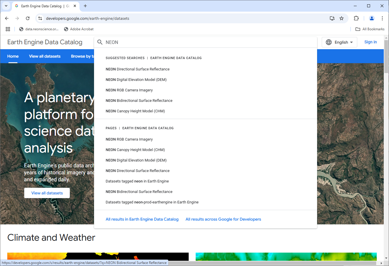
In the code editor, NEON datasets can be accessed through the projects/neon-prod-earthengine folder with an appended suffix of the Acronym and Revision Number, shown in the table below. For example, the Surface Directional Reflectance can be found under the path projects/neon-prod-earthengine/assets/HSI_REFL/001. The table below summarizes the GEE and NEON Data Portal IDs for each data product, and can be used as a reference for reading in AOP GEE datasets. You will learn how to access and read in these data products in the next part of this lesson.
| GEE Acronym/Revision | Data Product Name | Data Product ID |
|---|---|---|
| HSI_REFL/001 | Surface Directional Reflectance | DP3.30006.001 |
| HSI_REFL/002 | Surface Bidirectional Reflectance | DP3.30006.002 |
| RGB/001 | Red Green Blue (Camera Imagery) | DP3.30010.001 |
| DEM/001 | Digital Elevation Model (DSM/DTM) | DP3.30024.001 |
| CHM/001 | Ecosystem Structure (Canopy Height Model; CHM) | DP3.30015.001 |
| CNC/002 | Canopy Nitrogen Content (CNC) | DP3.30018.002 |
Get Started with Google Earth Engine
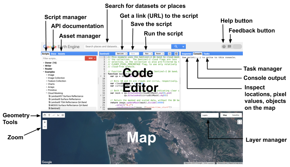
Once you have set up your Google Earth Engine account you can navigate to the Earth Engine Code Editor. The diagram below, from the Earth-Engine Playground, shows the main components of the code editor. If you have used other programming languages such as R, Python, or Matlab, this should look fairly similar to other Integrated Development Environments (IDEs) you may have worked with. The main difference is that this has an interactive map at the bottom, similar to Google Maps and Google Earth. We encourage you to play around with the interactive map, or explore the ee documentation, linked above, to gain familiarity with the various features.
Read AOP Data Collections into GEE
AOP data can currently be accessed through GEE through the projects/neon-prod-earthengine/assets/ folder. In the remainder of this lesson, we will look at the six available AOP datasets, or ImageCollections.
An ImageCollection is simply a group of images. To find publicly available datasets (primarily satellite data), you can explore the Earth Engine Data Catalog. The following steps will walk you through how to read in AOP Image Collections in the Code Editor.
In your code editor, copy and run the following lines of code to create 5 ImageCollection variables containing the Surface Directional Reflectance (HSI_REFL/001), Surface Bidirectional Reflectance (HSI_REFL/002), Camera Imagery (RGB), Canopy Height Model (CHM), and Digital Elevation Model (DEM) raster data sets.
// read in the AOP image collections
var refl001 = ee.ImageCollection('projects/neon-prod-earthengine/assets/HSI_REFL/001')

var refl002 = ee.ImageCollection('projects/neon-prod-earthengine/assets/HSI_REFL/002')

var rgb = ee.ImageCollection('projects/neon-prod-earthengine/assets/RGB/001')

var chm = ee.ImageCollection('projects/neon-prod-earthengine/assets/CHM/001')

var dem = ee.ImageCollection('projects/neon-prod-earthengine/assets/DEM/001')

var cnc = ee.ImageCollection('projects/neon-prod-earthengine/assets/CNC/002')
A few tips for the working in the Code Editor:
- In the left panel of the code editor, there is a Docs tab which includes API documentation on built in functions, showing the expected input arguments. We encourage you to refer to this documentation, as well as the GEE JavaScript Tutorial to familiarize yourself with GEE and the JavaScript programming language.
- If you have an error in your code, a red error message will show up in the Console (in the right panel), which tells you the line that failed.
- Save your code frequently! If you try to leave your code while it is unsaved, you will be prompted that there are unsaved changes in the editor.
When you Run the code above (by clicking on the Run above the code editor), you will notice that the lines of code become underlined in red, the same as you would see for a spelling error in most text editors. If you hover over each of the lines of codes, you will see a message pop up that prompts you to Convert the variable into an import record.

If you click Convert, the line of code will disappear and the variable will be imported into your session directly, and will show up at the top of the code editor. Go ahead and convert the variables for all three lines of code, so you should see the following. Tip: if you type Ctrl-z, you can re-generate the line of code, and the variable will still show up in the imported variables at the top of the editor. It is recommended to retain the code that reads in each variable, for reproducibility. If you don't do this, and wish to share this code with someone else, or run the code outside of your current code editor, the imported variables will not be saved and any subsequent code referring to this variable will result in an error message.

Note that each of these imported variables can now be expanded, using the arrow to the left of each. These variables now show associated information including type, id, and version.
Information about the image collections can also be found in a slightly more user-friendly format if you click on the blue link, eg. projects/neon-prod-earthengine/CHM/001. Below we'll show the window that pops-up when you click on the CHM link. We encourage you to explore all of the AOP datasets similarly. Note: You can also search for the NEON AOP image collections through the search bar on the Earth Engine Data Catalog webpage. The dataset page also contains all the information about the data product, eg. NEON Canopy Height Model (CHM).
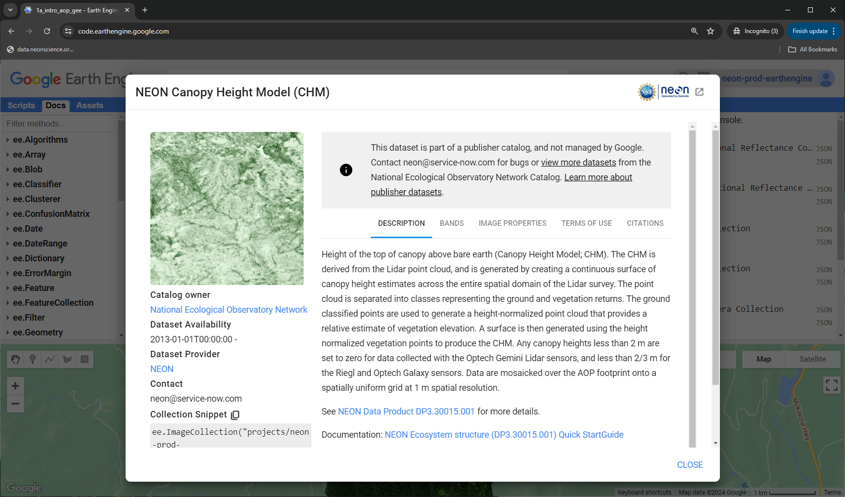
The end of the description includes a link to the Data Product landing page on the NEON Data Portal, as well as the Quick Start Guide, which includes links to all the documentation pertaining to this NEON data product, including the Algorithm Theoretical Basis Documents (ATBDs). Click on the other tabs to explore more about this data product. These tabs include DESCRIPTION, BANDS, IMAGE PROPERTIES, TERMS OF USE, AND CITATIONS.
TIP: You can also search for NEON data products through Code Editor by typing "NEON" in the search bar as shown below:

AOP GEE Data Availability
Since we are adding AOP data to GEE on a rolling basis, the first thing you may want to do after reading in the image collections is to determine which datasets are currently available on GEE. A quick way to do this is shown below:
// list available images in the NEON Surface Directional Reflectance Image Collection:
print('Images in the NEON Directional Refl Collection:',refl001.aggregate_array('system:index'));

// list available images in the NEON Surface Bidirectional Reflectance Image Collection:
print('Images in the NEON Bidirectional Refl Collection:',refl002.aggregate_array('system:index'));

// list available images in the NEON DEM image collection:
print('Images in the NEON DEM Collection:',dem.aggregate_array('system:index'));

// list available images in the NEON CHM image collection:
print('Images in the NEON CHM Collection:',chm.aggregate_array('system:index'));

// list available images in the NEON RGB image collection:
print('Images in the RGB Camera Collection:',rgb.aggregate_array('system:index'));

// list available images in the NEON Canopy Nitrogen (CNC) image collection:
print('NEON Images in the Canopy Nitrogen Collection',cnc.aggregate_array('system:index'));
In the Console tab to the right of the code, you will see a list of all available images. Expand each List to see the data available for each Image Collection. The names of the all the images follow the format YEAR_SITE_#, so you can identify the site and year of data this way. The number at the end is the Visit #; AOP typically visits each site 3 out of every 5 years, so the visit number indicates the cumulative number of times AOP has visited that site. Occasionally, AOP may re-visit a site twice in the same year. Note that the Canopy Nitrogen Image Collection only has a small number of images, this is because the dataset is newly available (first published in February 2026) and only a subset of data were published initially, to provide some initial examples for the community to review. Please see the NEON Data Notification: New Data Product: Canopy Nitrogen, Subset of Data Available for Community Review for more details.

Filter by Image Properties
Next, we can explore some filtering options to pull out individual images from an Image Collection. In the example shown below, we can filter by the date (.filterDate) by providing a date range, and filter by other properties, such as the NEON site code, using .filterMetadata. For this example we'll pull in an image from the NEON site Lyndon B. Johnson National Grassland NEON (CLBJ).
// Directional Reflectance (HSI_REFL/001)
// read in a single reflectance image at the NEON site CLBJ in 2021
var refl001_CLBJ_2021 = refl001
  .filterDate('2021-01-01', '2021-12-31') // filter by date - 2021
  .filterMetadata('NEON_SITE', 'equals', 'CLBJ') // filter by site
  .first(); // select the first one to pull out a single image
Explore Image Properties
Next let's take a look at the Image Properties.
// display the image properties
var clbj2021_refl001_props = refl001_CLBJ_2021.toDictionary();
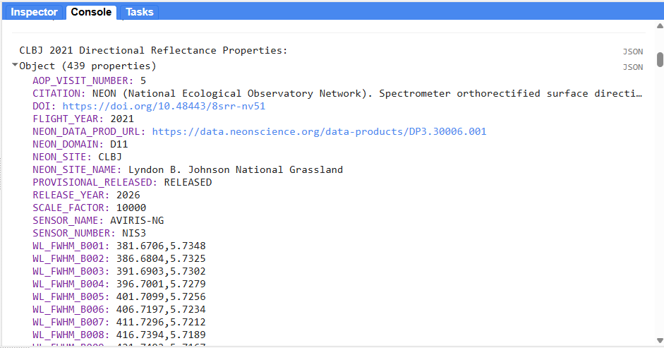
print('CLBJ 2021 Directional Reflectance Properties:',clbj2021_refl001_props);
Look in the Console for the properties, you can expand by clicking on the arrow to the left of the Object (439 properties). Here you can see some metadata about this image. Scroll down and you'll get to a number of properties starting with WL_FWHM_B###. These are the WaveLength (WL) and Full Width Half Max (FWHM) values, in nanometers, corresponding to each band (Bands 001 - 426). You may wish to refer to this wavelength information to determine which bands you wish to display, eg. if you want to show a false color image instead of a true color (RGB) image. For a full description of what each of the Image Properties mean, you can look at the IMAGE PROPERTIES tab as explained in the previous section, or find it in the Earth Engine Data Catalog.
Determine Release Tag, DOI, and Citation Information
When working with NEON data, whether downloaded from the Data Portal or on GEE, we always recommend checking whether the data are Provisional or Released, and also checking the release tag of the data. On GEE, this information is included in the image properties PROVISIONAL_RELEASED and RELEASE_YEAR. If the data is released, the property RELEASE_YEAR will display the year of the release. For data that has been released, the Digital Object Identifier (DOI) is also available in the DOI tag, and for all data there is a CITATION tag providing a suggested citation. The code chunk below shows how to display the release, DOI, and citation information for the CLBJ 2021 directional reflectance data.
// determine the release information for this image
// see https://www.neonscience.org/data-samples/data-management/data-revisions-releases
var clbj2021_refl001_release_status = clbj2021_refl001_props.select(['PROVISIONAL_RELEASED']);
print('CLBJ 2021 Directional Reflectance Release Status:', clbj2021_refl001_release_status)

var clbj2021_refl001_release_year = clbj2021_refl001_props.select(['RELEASE_YEAR']);
print('CLBJ 2021 Directional Reflectance Release Year:', clbj2021_refl001_release_year)

// digital object identifier (DOI)
var clbj2021_refl001_doi = clbj2021_refl001_props.select(['DOI']);
print('CLBJ 2021 Directional Refl DOI:', clbj2021_refl001_doi)

// citation - see https://www.neonscience.org/data/guidelines-policies/citing
var clbj2021_refl001_citation = clbj2021_refl001_props.select(['CITATION']);
print('CLBJ 2021 Directional Refl Citation:', clbj2021_refl001_citation)
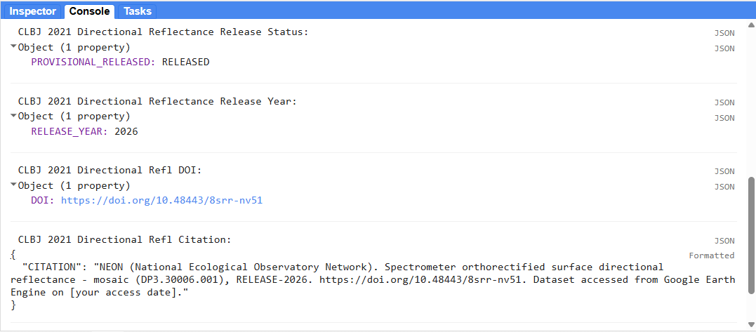
In this example, as of March 2026, the 2021 CLBJ directional reflectance data is part of RELEASE-2026.
See NEON's Data Product Revisions and Releases page as well as the Acknowledging and Citing NEON page for more information on releases and citing NEON data. There is a short period each year in January where AOP data on the NEON Data Portal may be in flux in preparation for an upcoming data release (which typically becomes available at the end of January each year). GEE datasets are planned to be kept up to date with the current NEON Data Release, however there may be a lag period between the annual release and data updates on GEE. Data on GEE should be updated to match the current release by the end of February each year. For current information around the release status and data quality issue notices, you can follow NEON Data Notifications.
Plot a True Color Image of Reflectance Data
Finally, let's plot a true color image (red-green-blue or RGB composite) of the reflectance data that we've read into the variable refl001_CBLJ_2021. To do this, first we pull out the RGB bands, set visualization parameters, center the map over the site, and then add the map using Map.addLayer. There are a couple ways you can center the Map to the location you want. One is to use Map.centerObject and you can provide the image you want to center; otherwise you can specify the latitude and longitude and use Map.setCenter(), shown in the commented-out lines at the bottom of the code chunk below.
// Add a Reflectance True Color Image Layer to the Map
// select the red, green, and blue bands
var refl001_CLBJ_2021_RGB = refl001_CLBJ_2021.select(['B053', 'B035', 'B019']);

// set visualization parameters
var refl_rgb_vis = {min: 0, max: 1260, gamma: 0.8};

// add this RGB layer to the Map and give it a title
Map.addLayer(refl001_CLBJ_2021_RGB, refl_rgb_vis, 'CLBJ 2021 Directional Reflectance RGB');

// use centerObject to center on the reflectance data, 13 is the zoom level
Map.centerObject(refl001_CLBJ_2021, 13)

// alternatively you could specify the lat / lon of the site, set zoom to 13
// you can find the field site lat/lon here https://www.neonscience.org/field-sites/clbj
// Map.setCenter(-97.57, 33.40, 13);
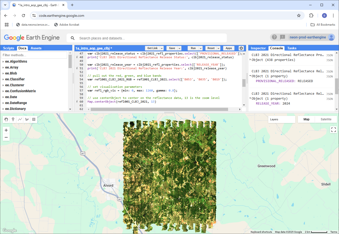
When you run the code you should now see the true color image on the map! You can zoom in and out and explore some of the other interactive options on your own. Toggle the Layers window in the upper right corner to view the layer and to change the histogram stretch and opacity of the image, if desired.
Compare Directional and Bidirectional Reflectance
Lastly, let's also look at a bidirectional data product at the same site, so you can explore some of the differences between the directional and bidirectional reflectance. We will also display the properties for this data.
// Bidirectional Reflectance (HSI_REFL/002)
// read in a bidirectional reflectance image at the NEON site CLBJ in 2022
var refl002_CLBJ_2022 = refl002
  .filterDate('2022-01-01', '2022-12-31') // filter by date - 2022
  .filterMetadata('NEON_SITE', 'equals', 'CLBJ') // filter by site
  .first(); // select the first one to pull out a single image

// display the bidirectional reflectance image properties
var clbj2022_refl002_props = refl002_CLBJ_2022.toDictionary()
print('CLBJ 2022 Bidirectional Reflectance Properties:',clbj2022_refl002_props);
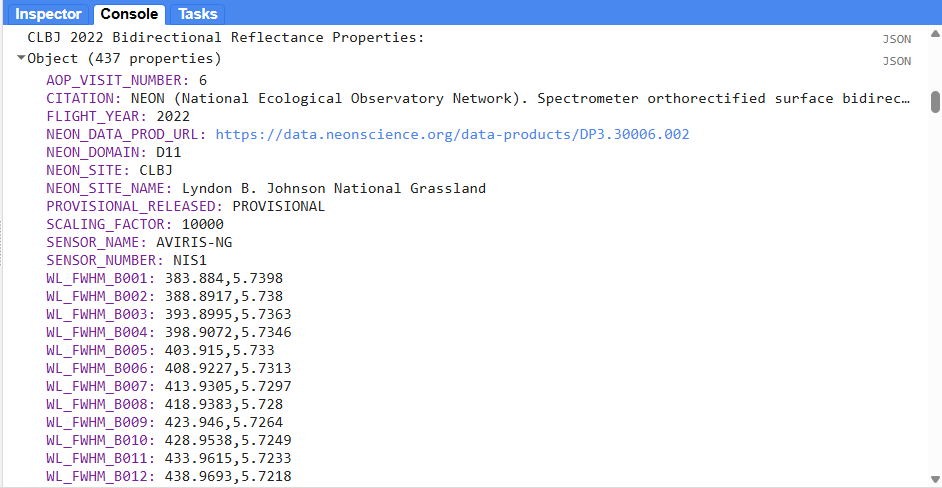
You'll notice that there are fewer properties for this bidirectional reflectance (HSI_REFL/002) image than we saw for the directional reflectance (HSI_REFL/001) data. The data are PROVISIONAL, and there are no RELEASE_YEAR or DOI properties. Bidirectional reflectance data will remain provisional in 2026, since it is a newer data product (as of 2024), and is planned to be incorporated into the upcoming RELEASE-2027.
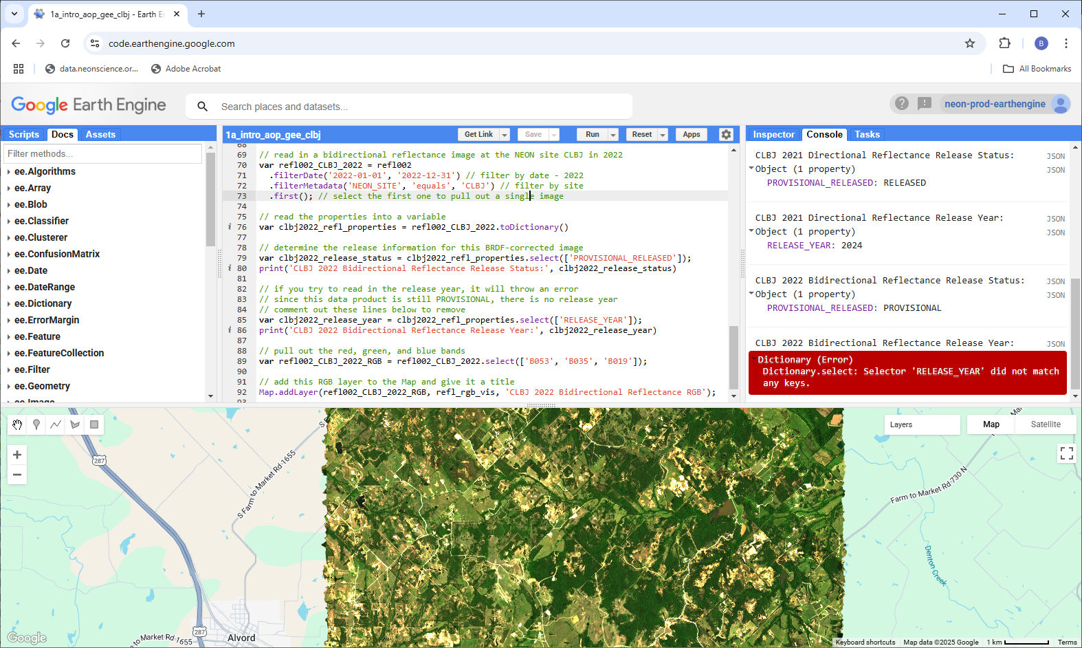
Tip: If your code has any errors they will display in the Console tab in red. For example, if you try to print out a property that does not exist (e.g. DOI and RELEASE_YEAR will not exist for any provisional data), then you will see an error in the console, as shown below. If your code is not running as expected, errors displayed in the Console can be helpful for troubleshooting, as they will tell you how and where your code failed. Print statements throughout the code can also be helpful.
Finally, let's add the bidirectional reflectance RGB (true color) image to the Map as a new layer.
// Add the Bidirectional Reflectance True Color (RGB) Image to the Map
// select the red, green, and blue bands
var refl002_CLBJ_2022_RGB = refl002_CLBJ_2022.select(['B053', 'B035', 'B019']);

// add this RGB layer to the Map
Map.addLayer(refl002_CLBJ_2022_RGB, refl_rgb_vis, 'CLBJ 2022 Bidirectional Reflectance RGB');
You can toggle between the two layers by selecting the Layers tab in the upper right corner of the Map window. Check and uncheck the two layers (2021 and 2022) to see the differences. You can also use the slider to the right of the layer name to make one layer partially transparent. What observations can you make about these two datasets?

The BRDF and topographic corrections typically visibly improve striping (or BRDF effects) between adjacent flightlines, as we can see with these datasets at CLBJ, where the 2022 bidirectional reflectance (left) looks much more seamless than the 2021 directional reflectance data (right), which has some visible vertical artifacts. For most NEON sites, the flight lines are oriented N-S so the stripes in the directional reflectance data will be vertical, but there are a few sites with slightly different flight plans.
A Quick Recap
You did it! You now have a basic understanding of the GEE Code Editor and its different components. You have also learned how to read a NEON AOP ImageCollection into a variable, import the variable into your session, and navigate through the ImageCollection Asset details to display information about the collection. You learned to read in an individual reflectance image, explore the image properties, and display a map of a true color image (RGB composite). And finally, you explored some of the differences between the directional and bidirectional (BRDF- and topographic corrected) reflectance data products at the site CLBJ.
It doesn't seem like we've done much so far, but this is a already great achievement! With just a few lines of code, you can import an entire AOP hyperspectral dataset, which in most other coding environments, is more involved. One of the major challenges to working with AOP reflectance data is its large data volume, which typically requires high-performance computing environments to read in the data, visualize, and analyze it. There are also limited open-source tools for working with hyperspectral data; many of the established software suites require proprietary (and often expensive) licenses. In this lesson, with minimal code, we have loaded spectral, lidar, and camera data covering an entire AOP site, and are ready to start exploring and analyzing the data in a free geospatial cloud-computing platform.
Get Lesson Code
Reflectance pre-processing: masking out bad weather data in GEE
Authors: Bridget M. Hass, John Musinsky
Last Updated: Jun 27, 2025
Since reflectance data is generated from a passive energy source (the sun), data collected in cloudy sky conditions are not directly comparable to data collected in clear-sky conditions, as overhead clouds can obscure the incoming light source. AOP aims to collect data only in optimal (<10% cloud-cover) weather conditions, but cannot always do so due to logistical constraints. The flight operators record the weather conditions during each flight, and this information is passed through to the final data product at the level of the flight line (as cloud conditions can change throughout the day). Cloud conditions are reported as green (<10% cloud cover), yellow (10-50% cloud cover), or red (>50% cloud cover). The figure below shows some examples of what the cloud conditions look like at different flights collected in the three different weather classes (green, yellow, and red).

Note that there is an important distinction between airborne and satellite reflectance data. Satellite data is collected in all weather conditions, and the clouds are below the sensor, so algorithms can be generated to filter out cloudy pixels. With aerial data, we have more control over when the data are collected, to a degree. However, clouds may be present overhead, if it were deemed necessary to collect in sub-optimal weather conditions. AOP typically will only collect in "red" sky conditions if we are running out of time in a Domain and the weather isn't forecasted to improve. Since the clouds won't appear in the actual data, maintaining this record of cloud conditions is essential for properly understanding the data, and using it for change detection or other research applications. For a more direct comparison of reflectance values, we recommend only working with the clear-weather data. This lesson outlines how to do this in GEE.
Objectives
After completing this activity, you will be able to:
- Extract and plot the weather quality indicator band from the Surface Directional Reflectance dataset
- Mask reflectance data to pull out only clear-weather data for a given site
- Explore other QA bands included in the Reflectance data set
Requirements
- Complete the following introductory AOP GEE tutorials:
- An understanding of hyperspectral data and AOP spectral data products. If this is your first time working with AOP hyperspectral data, we encourage you to start with:
- Intro to Working with Hyperspectral Remote Sensing Data in R. You do not need to follow along with the code in those lessons, but at least read through to gain a better understanding of NEON's hyperspectral data product.
Read in the AOP Surface Directional Reflectance 2019 Dataset at SOAP
For this exercise, we will read in directional reflectance data from the NEON site Soaproot Saddle (SOAP) collected in 2019:
// Filter image collection by date and site to pull out a single image
var soapSDR = ee.ImageCollection("projects/neon-prod-earthengine/assets/HSI_REFL/001")
  .filterDate('2019-01-01', '2019-12-31')
  .filterMetadata('NEON_SITE', 'equals', 'SOAP')
  .first();
Display the QA Bands
From the previous lesson, recall that the reflectance images include 442 bands. Bands 0-425 are the data bands, which store the spectral reflectance values for each wavelength recorded by the NEON Imaging Spectrometer (NIS). The remaining bands (426-441) contain metadata and QA information that are important for understanding and properly interpreting the hyperspectral data. The data bands all follow the naming convention B001, B002, ..., B426, and the QA bands have more descriptive names that start with something other than the letter "B", so we can use that information to extract the QA bands.
// Pull out and display only the qa bands (these all start with something other than B)
// '[^B].*' is a regular expression to pull out bands that don't start with B
var soapSDR_qa = soapSDR.select('[^B].*')
print('QA Bands',soapSDR_qa)
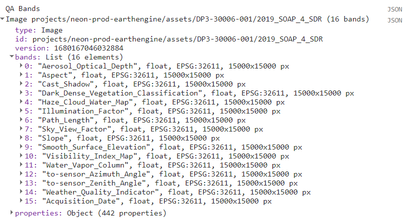
Most of these QA bands are inputs to and outputs from the Atmospheric Correction (ATCOR), the process which converts radiance to atmospherically corrected reflectance. We will elaborate on these QA bands further, and encourage you to read more details about these data in the NEON Imaging Spectrometer Radiance to Reflectance Algorithm Theoritical Basis Document. For the purposes of this exercise, we will focus on the Weather Quality Indicator band. Note that you can explore each of the QA bands, following similar steps below, adjusting the band names and values accordingly.
Read in the Weather_Quality_Indicator Band
The weather information, called Weather_Quality_Indicator is one of the most important pieces of QA information that is collected about the NIS data, as it has a direct impact on the reflectance values.
These next lines of code pull out the Weather_Quality_Indicator band, select the "green" weather data from that band, and apply a mask to keep only the clear-weather data, which is saved to the variable soapSDR_clear.
// Extract a single band Weather Quality QA layer
var soapWeather = soapSDR.select(['Weather_Quality_Indicator']);

// Select only the clear weather data (<10% cloud cover)
var soapClearWeather = soapWeather.eq(1); // 1 = 0-10% cloud cover

// Mask out all cloudy pixels from the SDR image
var soapSDR_clear = soapSDR.updateMask(soapClearWeather);
Plot the weather quality band data
For reference, we can plot the weather band data, using AOP's stop-light (red/yellow/green) color scheme, with the code below:
// center the map at the lat / lon of the site, set zoom to 12
Map.setCenter(-119.25, 37.06, 11);

// Define a palette for the weather - to match NEON AOP's weather color conventions
var gyrPalette = [
  '00ff00', // green (<10% cloud cover)
  'ffff00', // yellow (10-50% cloud cover)
  'ff0000' // red (>50% cloud cover)
];

// Display the weather band (cloud conditions) with the green-yellow-red palette
Map.addLayer(soapWeather,
             {min: 1, max: 3, palette: gyrPalette, opacity: 0.3},
             'SOAP 2019 Cloud Cover Map');
Plot the clear-weather reflectance data
Finally, we can plot a true-color image of only the clear-weather data, from soapSDR_clear that we created earlier:
// Create a 3-band cloud-free image
var soapSDR_RGB = soapSDR_clear.select(['B053', 'B035', 'B019']);

// Display the SDR image
Map.addLayer(soapSDR_RGB, {min:103, max:1160}, 'SOAP 2019 Reflectance RGB');
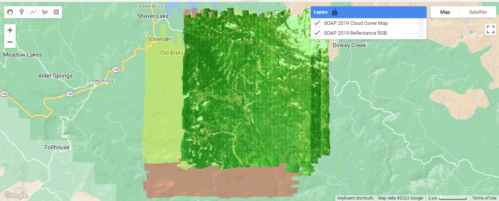
Plot acquisition dates
We can apply the same concepts to explore another one of the QA bands, this time let's look at the Acquisition_Date. This may be useful if you are trying to find the dates that correspond to field data you've collected, or you want to scale up to satellite data, for example. To determine the minimum and maximum dates, you can use reduceRegion with the reducer ee.Reducer.minMax() as follows. Then use these start and end date values in the visualization parameters.
Tip: You may not wish to show every layer by default if you are plotting many layers. You can choose not to display a layer by default by including a "0" as the last input of Map.addLayer. Once you run the code, to toggle the layer on, find the Layers tab in the upper right corner of the Map Window and check the box to the left of the layer you want to display. You can click on the lock icon to make it so that the Layers full display stays open (by default it minimizes).
// Extract acquisition dates QA band
var soapDates = soapSDR.select(['Acquisition_Date']);

// Get the minimum and maximum values of the soapDates band
var minMaxValues = soapDates.reduceRegion({reducer: ee.Reducer.minMax(),maxPixels: 1e10})
print('min and max dates', minMaxValues);

// Map acquisition dates, don't display layer by default
Map.addLayer(soapDates,
            {min:20190612, max:20190616, opacity: 0.5},
            'SOAP 2019 Acquisition Dates',0);
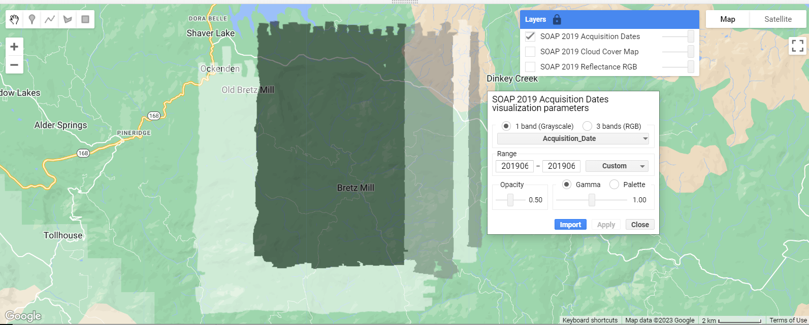
Other QA considerations
This lesson is intended to give you a quick introduction to some of the QA factors to consider when working with NEON AOP data, and is not meant to be comprehensive. When working with hyperspectral data, there are also invalid and noisy bands that you will likely want to remove before working with the full spectra (these bad bands are not unique to NEON hyperspectral data; for example NASA AVIRIS and EMIT hyperpsectral data have the same limitiations). Please see the lesson Plot spectral signatures of AOP Reflectance data in GEE for more details on these "bad bands". The Algorithm Theoretical Basis Documents (ATBDs) for the directional and bidirectional reflectance datasets, linked from the NEON Data Product Pages (DP3.30006.001, DP3.30006.002) and from the Quick Start Guides linked in the descriptions in the NEON Publisher Datasets pages on GEE, provide more comprehensive details on how these data products were derived and additional QA factors to consider. When pairing NEON data with satellite data, you will also need to factor in differences in how the datasets were processed, such as the atmospheric correction algorithm used, and other corrections that may or may not be applied (e.g. BRDF and topographic corrections) to both/all datasets you are integrating. If you can't find the information you need in the documentation, please reach out to NEON scientists using the NEON Contact Us form with any questions.
Recap
In this lesson you learned how to read in Weather Quality Information from the Reflectance QA bands in GEE. You learned to mask data to keep only the imagery collected in the clearest sky conditions (<10% cloud cover), and plot the three weather quality classes. You also learned how to find the other QA bands. Following a similar approach, you can explore each of the QA bands similarly. Filtering by the weather quality is an important first pre-processing step to working with NEON hyperspectral data, and is essential for interpreting the data and carrying out subsequent data analysis.
Get Lesson Code
Functions in Google Earth Engine (GEE)
Authors: Bridget Hass, John Musinsky
Last Updated: Jun 27, 2025
Writing a Function to Visualize AOP Reflectance Image Collections
In the earlier Reflectance pre-processing tutorial, we showed how to read in a band of data containing weather quality information and apply cloud-masking using that band. In this tutorial, we will show you a more simplified way of doing this, using functions so we can more easily apply that operation to an Image Collection. This is called "refactoring". In any coding language, if you notice you are writing very similar lines of code repeatedly, it may be an opportunity to create a function. As you become more proficient with GEE coding, it is good practice to start writing functions to make your scripts more readable and reproducible.
Objectives
After completing this activity, you will be able to:
- Understand the basic structure of functions in GEE (JavaScript API)
- Write and call a function to read in and display images from all available years in an AOP Reflectance Image Collection
- Write a function to add the weather quality layer to the map, and mask out cloudy data from an Reflectance Image Collection
Requirements
- An Earth Engine account. You can sign up for a non-commercial Earth Engine account here: https://code.earthengine.google.com/register
- A basic understanding of the GEE code editor and the GEE JavaScript API. These are introduced in the tutorials:
- A basic understanding of hyperspectral data and the AOP hyperspectral data products. If this is your first time working with AOP hyperspectral data, we encourage you to start with the Intro to Working with Hyperspectral Remote Sensing Data in R tutorial. You do not need to follow along with the R code in those lessons, but at least read through to gain a better understanding NEON's spectral data products.
Additional Resources
If this is your first time using GEE, we recommend checking out the Google Developers website, and working through some of the introductory tutorials. The links below are good places to start.
GEE Function and Mapping Syntax
Let's get started! First let's take a look at the syntax for writing user-defined functions in GEE. If you are familiar with other programming languages, this should look somewhat familiar. The function requires input argument(s) args and returns an output. Note: Do not try to run the two code chunks below, these are just to demonstrate the key components of a function and how you can call or "map" that function.
var functionName = function(args) {
  // do something with input args
  return output;
};
To call the function for a full image collection, you can use a map to apply the function to all items in a collection. This is outlined in the code chunk below.
// Map the function over the collection.
var newVariable = collection.map(myFunction);
Read in AOP Directional Reflectance Image Collection
First, we'll read in the AOP Directional Reflectance Image Collection at Jones Center At Ichauway (JERC).
// specify center location of the site (JERC)
var site_center = ee.Geometry.Point([-84.468623,31.194839])

// read in the AOP Directional Reflectance (HSI_REFL/001) Image Collection
// filter to the site_center
var sdr_col = ee.ImageCollection('projects/neon-prod-earthengine/assets/HSI_REFL/001')
  .filterBounds(site_center)

print('NEON AOP Directional Reflectance Image Collection',sdr_col)
Cloud Masking Function
Building off the example from the previous tutorial, we can write a simple function to apply cloud-masking to an Image Collection:
// Function to mask out poor-weather data, keeping only the <10% cloud cover weather data
function clearSDR(image) {
  // create a single band Weather Quality QA layer
  var weather_qa = image.select(['Weather_Quality_Indicator']);
  // WEATHER QUALITY INDICATOR = 1 is < 10% CLOUD COVER
  var clear_qa = weather_qa.eq(1);
  // mask out all cloudy pixels from the reflectance image
  return image.updateMask(clear_qa);
}
Then we can use .map() to apply this as follows:
// Use map to apply this function on all the NISImages and return a clear-weather collection
var sdr_cloudfree = sdr_col.map(clearSDR)
Function to Add Multiple Reflectance Layers to Map
For the next example, we will write a function to add a Map Layer for each Image in an Image collection. We'll provide the full script below, including the function addNISImage, with comments explaining what each part of the function does. Note that a helpful troubleshooting technique is to add in print statements if you are unsure what the code is returning. We have included some commented-out print statements in the function, which show the outputs (which would show up in the console tab).
For a little more detail on how this function was applied, refer to this GIS Stack Exchange Post: Add/display all images of my collection in google earth engine. When writing your own GEE code, the Google earth-engine developers pages may not always have an example of what you are trying to do, so stack overflow can be a valuable resource.
// Define visualization parameters for the reflectance data, showing a true-color image
// B053 ~ 642 nm, B035 ~ 552 nm , B019 ~ 472nm
var sdr_vis_params = {'min':0, 'max':1200, 'gamma': 0.9, 'bands': ['B053','B035','B019']};

// Function to display each NIS Image in the NEON AOP Image Collection
function addNISImage(image) {
  // get the system:id and convert to string
  var imageId = ee.Image(image.id);
  // get the system:id - this is an object on the server
  var sysID_serverObj = ee.String(imageId.get("system:id"));
  // getInfo() converts to string on the server
  var sysID_serverStr = sysID_serverObj.getInfo()
  // truncate the string to show only the fileName (NEON domain + site code + product code + year)
  var fileName = sysID_serverStr.slice(51,100);
  // print("fileName: "+fileName) // optionally print the file name, can uncomment

  // add this layer to the map using the true-color (RGB) visualization parameters
  Map.addLayer(imageId, sdr_vis_params, fileName + ' Refl RGB - All Flightlines')
}

// call the addNISimages function
sdr_col.evaluate(function(sdr_col) {
  sdr_col.features.map(addNISImage);
})

// Center the map on site and set zoom level (11)
Map.centerObject(site_center, 11);
Note that the first half of this function is just pulling out relevant information about the site in order to properly label the layer on the Map display. Note that defining this function alone will not display anything on the map, you will need to call (evaluate) the function.
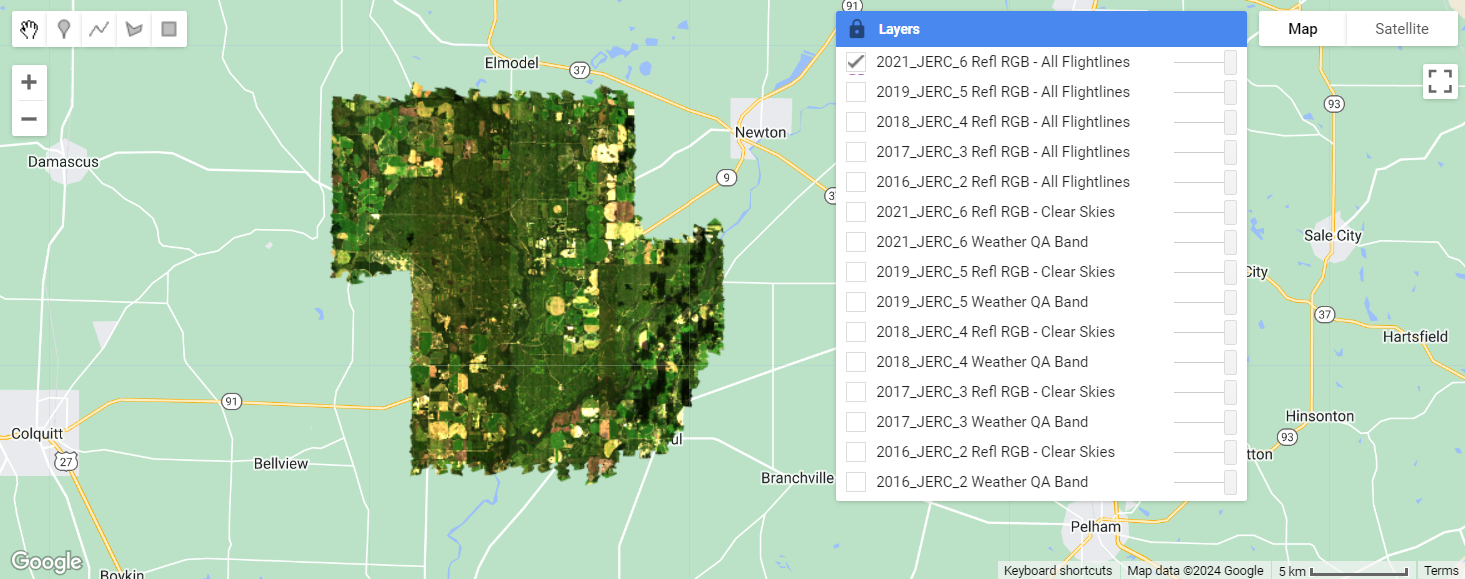
Function including Cloud-Masking and Weather QA Layers
Next we can build upon this function to include some other pre-processing steps, such as selecting the Weather_Quality_Indicator band, and masking the reflectance data to include only the clear-weather (<10% cloud cover) data. We can add the weather QA and clear-weather masked datasets as Layers to the Map.
// Define a palette for the weather - to match NEON AOP's weather color conventions
// This will be used in the visualization parameters for the Weather QA layer
// green (<10% cloud cover), yellow (10-50% cloud cover), red (>50% cloud cover)
var gyr_palette = ['green','yellow','red']

// Build upon the function to add a layer of the weather band, and
// mask out poor-weather data (>10% cloud cover), keeping only the clear weather (<10% cloud cover)
function addClearNISImages(image) {
  // get the system:id and convert to string
  var imageId = ee.Image(image.id);
  // get the system:id - this is an object on the server
  var sysID_serverObj = ee.String(imageId.get("system:id"));
  // getInfo() converts to string on the server
  var sysID_serverStr = sysID_serverObj.getInfo()
  // truncate the string to show only the fileName (NEON domain + site code + product code + year)
  var fileName = sysID_serverStr.slice(51,100); // optionally print, can uncomment

  // create a single band Weather Quality QA layer for 2016
  var weather_qa = imageId.select(['Weather_Quality_Indicator']);

  // apply the function from the beginning of this script to generate a cloud-free image
  // you can apply a function directly on a single image in this way
  var sdr_cloudfree = clearSDR(imageId)

  // add the weather QA bands to the map with the green-yellow-red palette
  Map.addLayer(weather_qa, {min: 1, max: 3, palette: gyr_palette, opacity: 0.3}, fileName + ' Weather QA Band')

  // add the clear weather reflectance layer to the map - the 0 means the layer won't be turned on by default
  Map.addLayer(sdr_cloudfree, sdr_vis_params, fileName + ' Refl RGB - Clear Skies', 0)
}

//call the clearNISImages function
sdr_col.evaluate(function(sdr_col) {
  sdr_col.features.map(addClearNISImages);
})

// Center the map on site and set zoom level (11)
Map.centerObject(site_center, 11);
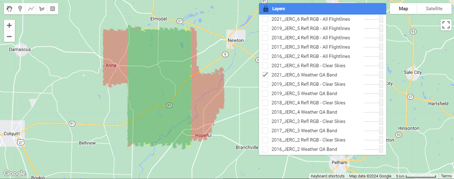
In the "Layers" tab, select and de-select the Map Layers to look at the data and the weather QA information for all of the years. This figure shows the weather quality information at JERC in 2019, where the data were collected in mixed cloud conditions. Flight operators prioritize flying the area over NEON plots in the best weather conditions when possible. As explained in the previous lesson, when working with AOP reflectance data, the weather conditions during the flights are one of the most important quality considerations.
Recap
This lesson showed how to make two functions that demonstrate using functional programming to add layers to a Map.
As explained in introduction-to-functional-programming, "Earth Engine uses a parallel processing system to carry out computation across a large number of machines...The use of for-loops is discouraged in Earth Engine. The same results can be achieved using a map() operation where you specify a function that can be independently applied to each element. This allows the system to distribute the processing to different machines." The examples presented in this lesson show how to make use of that map operation in lieu of a for loop.
Get Lesson Code
Functions to display AOP Reflectance Image Collections in GEE
Plot spectral signatures of AOP Reflectance data in GEE
Authors: Bridget Hass, John Musinsky
Last Updated: Jun 27, 2025
Objectives
After completing this activity, you will be able to:
- Read in and map a single AOP Hyperspectral reflectance image at a NEON site
- Link spectral band numbers to wavelength values
- Create an interactive plot to display the spectral signature of a given pixel upon clicking
Requirements
- Complete the following introductory AOP GEE tutorials:
- An understanding of hyperspectral data and AOP spectral data products. If this is your first time working with AOP hyperspectral data, we encourage you to start with the Intro to Working with Hyperspectral Remote Sensing Data tutorial. You do not need to follow along with the R code in those lessons, but at least read through to gain a better understanding NEON's spectral data products.
Read in the AOP Directional Reflectance Image
As should be familiar by now from the previous tutorials in this series, we'll start by pulling in the AOP data. For this exercise we will only read directional reflectance data from SOAP collected in 2021:
// Filter image collection by date and site
var soapSDR = ee.ImageCollection("projects/neon-prod-earthengine/assets/HSI_REFL/001")
  .filterDate('2021-01-01', '2021-12-31')
  .filterMetadata('NEON_SITE', 'equals', 'SOAP')
  .first();

// Create a 3-band true-color image
var soapSDR_RGB = soapSDR.select(['B053', 'B035', 'B019']);

// Display the SDR image
Map.addLayer(soapSDR_RGB, {min:103, max:1160}, 'SOAP 2021 Reflectance RGB');

// Center the map around the soapSDR_RGB object, set zoom to 12
Map.centerObject(soapSDR_RGB, 12);
Extract data bands
Next we will extract only the "data" bands in order to plot the spectral information. The reflectance data contains 426 data bands, and a number of QA/Metdata bands that provide additional information that can be useful in interpreting and analyzing the data (such as the Weather Quality Information). For plotting the spectra, we only need the data bands.
// Pull out only the data bands (these all start with B, eg. B001)
var soapSDR_data = soapSDR.select('B.*')
print('SOAP SDR Data',soapSDR_data)

// Read in the properties as a dictionary
var properties = soapSDR.toDictionary()
Extract wavelength information from the properties
Similar to the code above, we can use a regular expression to pull out the wavelength information from the properties. The wavelength and Full Width Half Max (FWHM) information is stored in the properties starting with WL_FWHM_B. These are stored as strings, so the nex step is to write a funciton that converts the string to a float, and only pulls out the center wavelength value (by splitting on the "," and pulling out only the first value). This is all we need for now, but if you needed the FWHM information, you could write a similar function. Lastly, we'll apply the function using GEE .map to pull out the wavelength information. We an then print some information about what we've extracted
// Select the WL_FWHM_B*** band properties (using regex)
var wl_fwhm_dict = properties.select(['WL_FWHM_B+\\d{3}']);

// Pull out the wavelength, fwhm values to a list
var wl_fwhm_list = wl_fwhm_dict.values()
print('Wavelength FWHM list:',wl_fwhm_list)

// Function to pull out the wavelength values only and convert the string to float
var get_wavelengths = function(x) {
  var str_split = ee.String(x).split(',')
  var first_elem = ee.Number.parse((str_split.get(0)))
  return first_elem
}

// apply the function to the wavelength full-width-half-max list
var wavelengths = wl_fwhm_list.map(get_wavelengths)

print('Wavelengths:',wavelengths)
print('# of data bands:',wavelengths.length())
Interactively plot the spectral signature of a pixel
Lastly, we'll create a plot in the Map panel, and use the Map.onClick function to create a spectral signature of a given pixel that you click on. Most of the code below specifies formatting, figure labels, etc.
// Create a panel to hold the spectral signature plot
var panel = ui.Panel();
panel.style().set({width: '600px',height: '300px',position: 'top-left'});
Map.add(panel);
Map.style().set('cursor', 'crosshair');

// Create a function to draw a chart when a user clicks on the map.
Map.onClick(function(coords) {
  panel.clear();
  var point = ee.Geometry.Point(coords.lon, coords.lat);
    wavelengths.evaluate(function(wvlnghts) {
      var chart = ui.Chart.image.regions({
        image: soapSDR_data,
        regions: point,
        scale: 1,
        seriesProperty: 'λ (nm)',
        xLabels: wavelengths.getInfo()
    });
    chart.setOptions({
      title: 'Reflectance',
      hAxis: {title: 'Wavelength (nm)',
      vAxis: {title: 'Reflectance'},
      gridlines: { count: 5 }}
    });
    // Create and update the location label
    var location = 'Longitude: ' + coords.lon.toFixed(2) + ' ' +
                   'Latitude: ' + coords.lat.toFixed(2);
    panel.widgets().set(1, ui.Label(location));
    panel.add(chart);
  })
});
When you run this code (linked at the bottom), you will see the SOAP 2021 directional reflectance layer show up in the Map panel, along with an empty white figure panel in the lower left corner. When you click anywhere in the reflectance image, the empty figure panel will be populated with the spectral signature of the pixel you clicked on.

QA Considerations - Bad and Noisy Bands
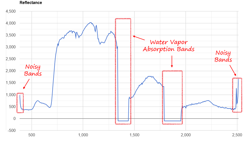
Let's zoom in on the spectral signature figure to take a closer look. Specifically, you can easily spot some QA considerations that are important to factor in if you intend to work with all 426 bands of data.
Water Vapor Band Windows
We can see from the spectral profile above that the reflectance values dip to below zero around ~1400 nm and ~1800 nm. These are water vapor band windows, resulting from water vapor which absorbs light between wavelengths 1340-1445 nm and 1790-1955 nm. The atmospheric correction that converts radiance to reflectance subsequently results in a spike at these two bands, and are invalid values. They are set to -100 for the reflectance data in GEE. For more details on these bands, please refer to the Plot a Spectral Signature from Reflectance Data in Python tutorial. If you are working with hyperspectral data downloaded from the NEON Data Portal, these water vapor band windows are not set to -100, so this is one difference between the reflectance datasets on GEE and the datasets and the original hdf5 reflectance datasets.
Noisy Bands
You may also notice that the reflectance values the beginning (~380 nm) and end (~2500 nm) of the wavelength range spike up, relative to the other nearby bands. These are not a feature of the actual data. The first and last bands are more prone to have noisy values due to imperfect calibration of the sensor at the lowest and highest reflectance bands. Best practice is to leave out the first and last 5-10 bands of data; you can inspect a spectral signature plot to determine how many bands to remove.
Recap
In this lesson you learned how to read in wavelength information from the Surface Directional Reflectance properties in GEE, created functions to convert from one data format to another, and created an interactive plot to visualize the spectral signature of a selected pixel. You can quickly see how GEE is a powerful tool for interactive data visualization and exploratory analysis.
Get Lesson Code
Wildfire Change Exploration Using AOP Reflectance and Canopy Height Data in GEE
Authors: John Musinsky, Stepan Bryleev, Bridget Hass
Last Updated: Jan 14, 2025
GEE is a great place to conduct exploratory analysis to better understand the datasets you are working with. In this lesson, we will show how to pull in AOP Surface Directional Reflectance (SDR) data, as well as the Ecosystem Structure (Canopy Height Model - CHM) data to look at interannual differences at the NEON site Great Smokey Mountains (GRSM), where the Chimney Tops 2 Fire broke out in late November 2016. NEON data over the GRSM site collected in June 2016 and October 2017 captures most of the burned area and presents a unique opportunity to study wildfire effects on the ecosystem and analysis of post-wildfire vegetation recovery. In this lesson, we will calculate the differenced Normalized Burn Ratio (dNBR) between 2017 and 2016, and also create a CHM difference raster to highlight vegetation structure differences in the burned area. We will also pull in Landsat satellite data and create a time-series of the NBR within the burn perimeter to look at annual differences.
Using remote sensing data to better understand wildfire impacts is an active area of research. In April 2023, Park and Sim published an Open Access paper titled "Characterizing spatial burn severity patterns of 2016 Chimney Tops 2 fire using multi-temporal Landsat and NEON LiDAR data". We encourage you to read this paper for an example of wildfire research using AOP remote sensing and satellite data. This lesson provides an introduction to conducting this sort of analysis in Google Earth Engine.
Objectives
After completing this activity, you will be able to:
- Write GEE functions to display map images of AOP SDR and CHM data.
- Use reducers to calculate statistics over an area.
- Conduct exploratory analysis in GEE to understand wildfire dynamics.
You will gain familiarity with:
- User-defined GEE functions
- Zonal statistics
Requirements
- An Earth Engine account. You can sign up for an Earth Engine account here: https://earthengine.google.com/new_signup/.
- A basic understanding of the GEE code editor and the GEE JavaScript API.
- Optionally, complete the previous GEE tutorials in this tutorial series:
Additional Resources
If this is your first time using GEE, we recommend starting on the Google Developers website, and working through some of the introductory tutorials. The links below are good places to start.
Functions to Read in SDR and CHM Image Collections
Let's get started. The code in the beginning of this lesson should look familiar from the previous tutorials in this series. In this first chunk of code, we will the center location of GRSM, and read in the fire perimeter as a FeatureCollection. We will also define some custom color palettes that are pulled from GitHub gee-community/ee-palettes. These custom palettes are not required, but will help make a nice visualization.
// Specify center location and flight box for GRSM (https://www.neonscience.org/field-sites/grsm)
var site_center = ee.Geometry.Point([-83.5, 35.7])

// Read in the Chimney Tops fire perimeter shapefile
var ct_fire_boundary = ee.FeatureCollection('projects/neon-sandbox-dataflow-ee/assets/chimney_tops_fire')

// Custom color palettes - https://github.com/gee-community/ee-palettes
var palettes = require('users/gena/packages:palettes');
var chm_palette = palettes.colorbrewer.Greens[5]
var dchm_palette = palettes.colorbrewer.RdBu[7]
var dnbr_palette = palettes.colorbrewer.RdYlGn[9].reverse()
Next, we'll read in the SDR image collection, and then write a function to mask out the cloudy weather data, and use the map feature to apply this to our SDR collection at GRSM.
// Read in the SDR Image Collection at GRSM
var grsm_sdr_col = ee.ImageCollection('projects/neon-prod-earthengine/assets/HSI_REFL/001')
  .filterBounds(site_center)

// Function to mask out poor-weather data, keeping only the <10% cloud cover weather data
function clearSDR(image) {
  // create a single band Weather Quality QA layer
  var weather_qa = image.select(['Weather_Quality_Indicator']);
  // WEATHER QUALITY INDICATOR = 1 is < 10% CLOUD COVER
  var clear_qa = weather_qa.eq(1);
  // mask out all cloudy pixels from the SDR image
  return image.updateMask(clear_qa);
}

// Use map to apply the clearSDR function to the SDR collection and return a clear-weather subset of the data
var grsm_sdr_cloudfree = grsm_sdr_col.map(clearSDR)
Next let's write a function to display the NIS images from 2016, 2017, and 2021 in GEE. For more details on how this function works, you can refer to the tutorial Functions in Google Earth Engine (GEE).
// Function to display individual (yearly) SDR Images
function addSDRImage(image) {
  var image_id = ee.Image(image.id); // get the system:id and convert to string
  var sys_id = ee.String(image_id.get("system:id")).getInfo();  // get the system:id - this is an object on the server
  var filename = sys_id.slice(52,100); // extract the fileName (NEON domain + site code + product code + year)
  var image_rgb = image_id.select(['B053', 'B035', 'B019']);  // select only RGB bands for display

  Map.addLayer(image_rgb, {min:220, max:1600}, filename, 1)   // add RGB composite to the map
}

// call the addNISimages function to add SDR layers to map
grsm_sdr_col.evaluate(function(grsm_sdr_col) {
  grsm_sdr_col.features.map(addSDRImage);
})
Next we can create a similar function for reading in the CHM dataset over all the years. The main differences between this function and the previous one are that 1) it is set to display a single band image, and 2) instead of hard-coding in the minimum and maximum values to display, we dynamically determine them from the data itself, so it will scale appropriately.
// Read in the CHM Image collection at GRSM
var grsm_chm_col =  ee.ImageCollection('projects/neon-prod-earthengine/assets/CHM/001')
  .filterBounds(site_center)

// Function to display Single Band Images setting display range to linear 2%
function addSingleBandImage(image) { // display each image in collection
  var image_id = ee.Image(image.id); // get the system:id and convert to string
  var sys_id = ee.String(image_id.get("system:id")).getInfo();
  var filename = sys_id.slice(52,100); // extract the fileName (NEON domain + site code + product code + year)

  // Dynamically determine the range of data to display
  // Sets color scale to show all but lowest/highest 2% of data
  var pct_clip = image_id.reduceRegion({
    reducer: ee.Reducer.percentile([2, 98]),
    scale: 10,
    maxPixels: 3e7});

  var keys = pct_clip.keys();
  var pct02 = ee.Number(pct_clip.get(keys.get(0))).round().getInfo()
  var pct98 = ee.Number(pct_clip.get(keys.get(1))).round().getInfo()

  Map.addLayer(image_id, {min:pct02, max:pct98, palette: chm_palette}, filename, 0)
}

// Call the addSingleBandImage function to add CHM layers to map
grsm_chm_col.evaluate(function(grsm_chm_col) {
  grsm_chm_col.features.map(addSingleBandImage);
})

// Center the map on GRSM and set zoom level to 12
Map.setCenter(-83.5, 35.6, 12);
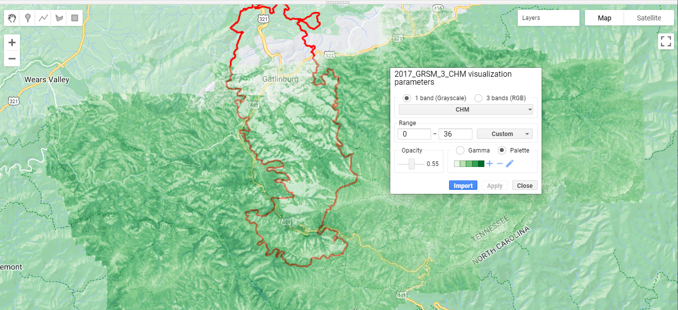
Now that you've read in these two datasets (SDR and CHM) over all the years of available data, we encourage you to explore the different layers and see what you notice! Toggle between the layers, play with the opacity. Visual inspection is an important first step in exploratory analysis - see if you can recognize patterns and form new questions based off what you see.
CHM Difference Layers
Next let's create a new raster layer of the difference between the CHMs from 2 different years.
// Difference the CHMs from 2017 and 2016 and 2021
var grsm_chm2021 = grsm_chm_col.filterDate('2021-01-01', '2021-12-31').first();
var grsm_chm2017 = grsm_chm_col.filterDate('2017-01-01', '2017-12-31').first();
var grsm_chm2016 = grsm_chm_col.filterDate('2016-01-01', '2016-12-31').first();

// Subtract the CHMs to create difference CHM rasters
var chm_diff_2017_2016 = grsm_chm2017.subtract(grsm_chm2016);
var chm_diff_2021_2017 = grsm_chm2021.subtract(grsm_chm2017);
var chm_diff_2021_2016 = grsm_chm2021.subtract(grsm_chm2016);

// Display the first CHM difference raster (2017-2016) and add as a layer to the Map
print('CHM Difference 2017-2016',chm_diff_2017_2016)

Map.addLayer(chm_diff_2017_2016, {min: -10, max: 10, palette: dchm_palette}, 'CHM diff 2017-2016');
CHM Difference Stats and Histograms
Next let's calculate the mean difference in Canopy Height inside the fire perimeter for the various years. We'll also plot histograms of the CHM differences.
// Calculate the mean dCHM between the various years:
print('Mean dCHM in the Chimney Tops Fire Perimeter')

print('Mean dCHM 2017-2016',chm_diff_2017_2016.reduceRegion({
      reducer: ee.Reducer.mean(),
      geometry: ct_fire_boundary,
      scale: 30}));

print('Mean dCHM 2021-2017',chm_diff_2021_2017.reduceRegion({
      reducer: ee.Reducer.mean(),
      geometry: ct_fire_boundary,
      scale: 30}));

print('Mean dCHM 2021-2016',chm_diff_2021_2016.reduceRegion({
      reducer: ee.Reducer.mean(),
      geometry: ct_fire_boundary,
      scale: 30}));
In the console, if you expand the objects, you can see that from 2016-2017, there was a net loss in canopy height of ~6.6m, and between 2017-2021 there was a net growth of ~3m, suggesting a considerable amount of re-growth in the 5 years after the fire.
We can also look at the histograms of the CHM differences to provide a little more information about the ecosystem structure dynamics immediately after the fire and in the subsequent years. To plot histograms, first write a function to create a histogram given a difference CHM raster (calculated above) and a string of the years that are being differenced, as inputs. The string is just used to include in the histogram chart title.
// Function to create histogram charts for each CHM difference layer, clipped by the chimney tops fire perimeter
function chmDiffHist(img,years_str) {
  var hist =
      ui.Chart.image.histogram({image: img.clip(ct_fire_boundary), region: ct_fire_boundary, scale: 50})
          .setOptions({title: 'CHM Difference Histogram ' + years_str,
                      hAxis: {title: 'CHM Difference (m)',titleTextStyle: {italic: false, bold: true},},
                      vAxis: {title: 'Count', titleTextStyle: {italic: false, bold: true}},});
  return hist
}

// Apply the function to the three CHM difference rasters
var chm_diff_hist_2017_2016 = chmDiffHist(chm_diff_2017_2016,'2017-2016')
var chm_diff_hist_2021_2016 = chmDiffHist(chm_diff_2021_2016,'2021-2016')
var chm_diff_hist_2021_2017 = chmDiffHist(chm_diff_2021_2017,'2021-2017')

// Display the CHM difference histograms charts on the Console
print(chm_diff_hist_2017_2016);
print(chm_diff_hist_2021_2017);
print(chm_diff_hist_2021_2016);
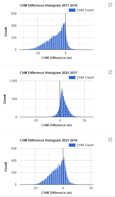
On your own, try to interpret what these difference histograms are showing.
Normalized Burn Ratio (NBR)
Last but not least, we can take a quick look at the NBR and dNBR. Refer to the CU Earth Lab dNBR Lesson for a nice explanation of this metric in the context of multispectral satellite data.
// Read in clear SDR images at GRSM in 2016, 2017, and 2021
var grsm_sdr2016_clear = grsm_sdr_cloudfree.filterDate('2016-01-01', '2016-12-31').first()
var grsm_sdr2017_clear = grsm_sdr_cloudfree.filterDate('2017-01-01', '2017-12-31').first();
var grsm_sdr2021_clear = grsm_sdr_cloudfree.filterDate('2021-01-01', '2021-12-31').first();

//------------------------- Normalized Difference Burn Ratio ----------------------------
// The normalized burn ratio (NBR) is a normalized difference index using the shortwave-infrared (SWIR) and near-infrared (NIR) portions of the electromagnetic spectrum. dNBR can be used as a metric to map fire extent and burn severity when calculating the difference between pre and post fire conditions.

// calculate NBR for the 3 years
// B097: B365:
var sdr_pre_nbr_2016 = grsm_sdr2016_clear.normalizedDifference(['B097', 'B365']);
var sdr_post_nbr_2017 = grsm_sdr2017_clear.normalizedDifference(['B097', 'B365']);
var sdr_post_nbr_2021 = grsm_sdr2021_clear.normalizedDifference(['B097', 'B365']);

// calculate dNBR 2016-2017 and 2016-2021
var sdr_dNBR_2016_2017 = sdr_pre_nbr_2016
                            .subtract(sdr_post_nbr_2017)
                            .clip(ct_fire_boundary);

var sdr_dNBR_2016_2021 = sdr_pre_nbr_2016
                            .subtract(sdr_post_nbr_2021)
                            .clip(ct_fire_boundary);

// Remove comment-symbols (//) below to display pre- and post-fire NBR as layers
// Map.addLayer(sdr_pre_nbr_2016, {min: -1, max: 1, palette: red_ylw_grn}, 'Pre-fire (June 2016) Normalized Burn Ratio');
// Map.addLayer(sdr_post_nbr_2017, {min: -1, max: 1, palette: red_ylw_grn}, 'Post-fire (Oct 2017) Normalized Burn Ratio');
// Map.addLayer(sdr_post_nbr_2021, {min: -1, max: 1, palette: red_ylw_grn}, 'Post-fire (June 2021) Normalized Burn Ratio');

// add dNBR layers
Map.addLayer(sdr_dNBR_2016_2017, {min: -1, max: 1, palette: dnbr_palette}, 'dNBR 2016-2017');
Map.addLayer(sdr_dNBR_2016_2021, {min: -1, max: 1, palette: dnbr_palette}, 'dNBR 2016-2021');
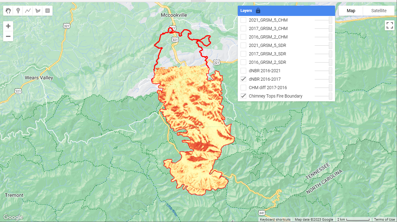
The differenced Normalized Burn Ratio (dNBR) does a great job of highlighting the burned areas (in red).
On your own, we encourage you to dig into the code from this tutorial and expand upon it according to your scientific interests. Think of some questions you have about this dataset and think about how you might answer it using GEE. Modify these functions or try writing your own function to answer your question(s). For example, try out different reducers to compile other statistics to summarize the CHM and NBR differences, or see if there are any other datasets that you could bring in to expand your analysis. This is just the starting point!
Get Lesson Code
NDVI Time Series using AOP Reflectance and Landsat 8 Data in GEE
Authors: Bridget M. Hass, John Musinsky
Last Updated: Jan 14, 2025
In this lesson, we'll continue to use the Great Smokey Mountains site as an example, this time creating a time series of the mean NDVI within the Chimney Tops 2 Fire perimeter between 2016-2022. We will plot this along with the NDVI time-series derived from Landsat 8 data, and use this to fill in some more detailed temporal information.
AOP strives to collect every site during peak-greenness, when the predominant vegetation is most photosynthetically active. This is so that when comparing data from year to year, the differences are due to actual changes and not just due to the time of year. This is not always possible, so it's important to consider the time of year when you are conducting your analysis.
Objectives
After completing this activity, you will be able to:
- Compare AOP data to Landsat 8 data
- Create an NDVI time series using two sets of data with different timestamps
- Understand the trade-offs in different kinds of resolutions (spatial, spectral, and temporal)
Requirements
- Register for an Earth Engine account; if you haven't already done this, you can here.
- A basic understanding of the GEE code editor and the GEE JavaScript API.
- Optionally, complete the previous GEE tutorials in this tutorial series:
Additional Resources
If this is your first time using GEE, we recommend starting on the Google Developers website, and working through some of the introductory tutorials. The links below are good places to start.
Read in AOP and Landsat 8 Surface Reflectance Image Collections
First read in the AOP directional reflectance data and the Landsat 8 data, filtering the AOP data by the site (GRSM) and filtering the Landsat data by the Chimney Tops Fire region of interest, and by date.
// Specify center location for GRSM
// Site lat/lon can be found on the field site page: https://www.neonscience.org/field-sites/grsm
var site_center = ee.Geometry.Point([-83.5, 35.7]);

// Create region of interest (roi)
var roi = ee.FeatureCollection('projects/neon-sandbox-dataflow-ee/assets/chimney_tops_fire')

// Read in the reflectance Image Collection
var sdr_col = ee.ImageCollection('projects/neon-prod-earthengine/assets/HSI_REFL/001')
  .filterMetadata('NEON_SITE', 'equals', 'GRSM')

// Read in Landsat 8 Surface Reflectance Image Collection
var l8sr = ee.ImageCollection('LANDSAT/LC08/C02/T1_L2')
                .filterBounds(roi)
                .filter(ee.Filter.calendarRange(2016, 2022, 'year'));
Cloud Mask Function for Landsat 8 Data
Next we can create a function to pre-process the Landsat 8 data, which applies scaling and cloud / saturated data masking. Don't worry too much about the details here, but the main thing to be aware of is that different satellite image collections handle the QA information differently. Landsat (and other satellites) often use something called "bitmasking" to store QA information, which is a space-efficient storage method. This cloud-masking function can be found on the earthengine-api GitHub examples here.
// cloud masking function for Landsat 8 Collection 2
function maskL8sr(image) {

  var qaMask = image.select('QA_PIXEL').bitwiseAnd(parseInt('11111', 2)).eq(0);
  var saturationMask = image.select('QA_RADSAT').eq(0);

  // Apply the scaling factors to the appropriate bands.
  var opticalBands = image.select('SR_B.').multiply(0.0000275).add(-0.2);
  var thermalBands = image.select('ST_B.*').multiply(0.00341802).add(149.0);

  // Replace the original bands with the scaled ones and apply the masks.
  return image.addBands(opticalBands, null, true)
      .addBands(thermalBands, null, true)
      .updateMask(qaMask)
      .updateMask(saturationMask);
}

// Apply the cloud masking function
l8sr = l8sr.filterBounds(roi).map(maskL8sr)
Merge AOP and Landsat 8 NDVI Collections
Next we can plot the two datasets on the same chart. This code was modified from this Stack Overflow post.
// compute ndvi bands to add to each collection
var addL8Bands = function(image){
  var l8_ndvi = image.normalizedDifference(['SR_B5','SR_B4']).rename('l8_ndvi')
  var aop_ndvi = ee.Image().rename('aop_ndvi')
  return image.addBands(l8_ndvi).addBands(aop_ndvi)
}

var addAOPBands = function(image){
  var aop_ndvi = image.normalizedDifference(['B097', 'B055']).rename('aop_ndvi')
  var l8_ndvi = ee.Image().rename('l8_ndvi')
  return image.addBands(aop_ndvi).addBands(l8_ndvi)
}

l8sr = l8sr.map(addL8Bands)
sdr_col = sdr_col.map(addAOPBands)

print('NIS Images',sdr_col)

// merge the collections
var merged = l8sr.merge(sdr_col).select(['l8_ndvi', 'aop_ndvi'])
Plot NDVI Time Series
Lastly we can create and plot (print) the time-series chart. Most of this is just setting the chart style.
// Set chart style properties.
// https://developers.google.com/earth-engine/guides/charts_style
var chartStyle = {
  title: 'NDVI at Chimney Tops Fire ROI - AOP + Landsat 8',
  hAxis: {
    title: 'Date',
    titleTextStyle: {italic: false, bold: true},
    gridlines: {color: 'FFFFFF'}
  },
  vAxis: {
    title: 'Mean NDVI',
    titleTextStyle: {italic: false, bold: true},
    gridlines: {color: 'FFFFFF'},
    format: 'short',
    baselineColor: 'FFFFFF'
  },
  series: {
    0: {lineWidth: 3, color: 'E37D05', pointSize: 7},
    1: {lineWidth: 3, color: '1D6B99'}
  },
  chartArea: {backgroundColor: 'EBEBEB'}
};

// Plot the merged (AOP + Landsat 8) Image Collection NDVI Time Series
var ndvi_timeseries = ui.Chart.image.series({
  imageCollection: merged,
  region: roi,
  reducer: ee.Reducer.mean(),
  scale: 30 // 	Scale to use with the reducer in meters
}).setOptions(chartStyle);

print(ndvi_timeseries)
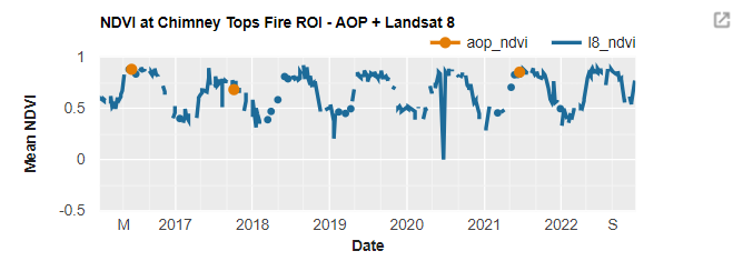
This figure demonstrates some important points. First, we can see that there is fairly good alignment between the mean NDVI calculated from AOP reflectance data and Landsat 8 at these times. While the Airborne Observation Platform seeks to collect data in peak green conditions, this is not always possible due to logistical or other constraints. For this site, one of the AOP collections in 2017 was in October, past peak-greenness, and the leaves already started senescing in some areas. Generating a time-series plot like this can help highlight the data in the context of the larger temporal trends. In this example, the NDVI time-series generated from Landsat 8 shows strong seasonal trends, as you might expect. This brings us to the second point: while AOP data has very high spectral (426 bands) and spatial (1m) resolution, the temporal resolution (site visits 3 out of every 5 years) may not provide enough temporal coverage, depending on your research application. This is where scaling with satellite data - either to expand your analysis to a larger area, or to achieve a more comprehensive temporal picture - can be useful. This tutorial demonstrates a simple example of scaling with satellite data to fill in temporal resolution for a basic NDVI calculation, and shows how GEE makes this sort of scalable analysis much simpler!