Explore NEON biodiversity data using ecocomDP

Introduction

In ecological synthesis projects, tasks related to finding, accessing, and vetting datasets to include in an analysis often creates an enormous time sink. However, it is crucial that investigators understand the structure of and assumptions behind each of the datasets included in a study. In this code-along tutorial, we will learn about tools available in the ecocomDP package for R to facilitate this initial data discovery, wrangling, and vetting process for datasets representing communities of organisms.

"ecocomDP" is both the name of an R package and a data model.

The data model can be described as "a dataset design pattern for ecological community data to facilitate synthesis and reuse". Because this data model is intended for use with community data, observations are expected to be measures of species abundance, biomass, or similar. However, some ecocomDP datasets report occurrences. The motivation for applying the ecocomDP data pattern to both NEON biodiversity data products and EDI data packages, including data from the US Long Term Ecological Research (LTER) Network and Macrosystems Biology projects, is to make these data discoverable and accessible through a single data search tool and to be delivered in a standard format. Functions in the ecocomDP package provide tools to maniuplate and visualize ecocomDP formatted data objects in R. We are also in the process of developing tools to easily convert ecocomDP data packages to Darwin Core Archives (DwC-A, event core) for submission to GBIF to further facilitate NEON and LTER data discovery.

For more information on ecocomDP, see:

• The GitHub repo: EDIorg/ecocomDP
• The website: ediorg.github.io/ecocomDP

In this lesson, we will learn how to find and access ecological community datasets provided by the National Ecological Observatory Network (NEON) and the Environmental Data Initiative (EDI).

Exercises in this lesson will cover:

• How to access NEON data and supporting information using the NEON data portal
• How to import NEON data into your R session
• An example of data wrangling necessary to use a NEON organismal dataset
• How to access an EDI dataset and import it into your R session
• How to find and access a NEON dataset using ecocomDP
• How to use ecocomDP plotting functions
• How to access an EDI dataset using ecocomDP
• How to compare multiple ecocomDP formatted datasets
• Options for working with data in the CyVerse Data Store

Things you'll need to complete this tutorial

1. R Programming Language

You will need some familiarity with the R programming language to complete this tutorial and we recommend you use a version of the RStudio IDE. In this tutorial, we will describe how to access an instance of RStudio with all the required packages pre-installed via your web browser using the Visual Interactive Computing Environment (VICE) provided in the CyVerse Discovery Environment. Alternatively, you can also complete most of the exercises in this tutorial using a locally installed version of R and RStudio.

2. [OPTIONAL] A NEON user account and API token

We recommend that you sign up for a NEON user account and set up an API token to access NEON data following the instructions outlined in this tutorial. This is not required. You can download NEON data without a token, but using an API token will enable faster download speeds.

3. [OPTIONAL] Create a CyVerse account and request access to VICE

To use the cloud computing resources available through VICE, you will need to create a CyVerse account and request access to VICE ahead of time (see below). If you choose this option, all of the required R packages should already be installed and you will be able to easily access and/or share large datasets in the CyVerse Data Store

4. R packages required for this tutorial

Prior to starting the tutorial, ensure that the following packages are installed (NOTE: these packages should be pre-installed if you are using the VICE RStudio app):

• tidyverse: install.packages("tidyverse")
• neonUtilities: install.packages("neonUtilities")
• ecocomDP: install.packages("ecocomDP")
• vegan: install.packages("vegan")

More on Packages in R – Adapted from Software Carpentry.

Load libraries and prepare workspace

First, we will load all necessary libraries into our R environment. If you are not using the RStudio VICE app with the packages pre-installed and you have not already installed these libraries, please see the "R packages required for this tutorial" section above.

# clean out workspace



#rm(list = ls()) # OPTIONAL - clear out your environment

#gc()            # Uncomment these lines if desired



# load packages

library(tidyverse)

library(neonUtilities)

library(ecocomDP)

This code chunk also includes two optional lines for clearing out your environment, which will erase all of the variables and data that are currently loaded in your R session. This is a good practice for many reasons, but only do this if you are completely sure that you won't be losing any important information!

Also, consider using a NEON API token. This will allow you increased download speeds and helps NEON anonymously track data usage statistics, which helps us optimize our data delivery platforms, and informs our monthly and annual reporting to our funding agency, the National Science Foundation. Please consider signing up for a NEON data user account, and using your token as described in this tutorial here. The linked tutorial describes a couple options for using your API token if you are running code locally. Below, we provide instructions for setting up an environmental variable to use your API token with the VICE cloud.

Now that our workspace is prepared, let's look at some data.

How to get data from the source (NEON and EDI data portals)

EXAMPLE 1: NEON benthic macroinvertebrates

First, take a look at the data product landing page: https://data.neonscience.org/data-products/DP1.20120.001

Note the abstract, information on latency, the design description, links to relevant documentation, the issue log, and the data availability matrix. Use the data availability matrix to help guide your choice of NEON sites and dates to include in your data download.

You can download the data using the web interface (see this video), but today we will learn how to download data from the NEON Data Portal API in an R session.

How to download a NEON data product using neonUtilities

NEON data are delivered in site-month chunks, so it is necessary to "stack" the data after you have downloaded all of your desired site-month data packages. However, you do not need to worry about data stacking because the NEON staff have developed the neonUtilities R package, which provides wrapper functions to interact with the NEON Data Portal API and appropriately unzip and stack the data tables so that they are more user friendly. For more details, see this tutorial on NEON data stacking. Here we use the loadByProduct function to download NEON macroinvertebrate data from two sites from 2017-2019. The loadByProduct function will extract the zip files, stack the data, and load it into your R environment. See this cheatsheet for more information on neonUtilities.

# Download NEON aquatic macroinvertebrate data from the NEON data portal API

# Should take < 1 minute

all_tabs_inv <- neonUtilities::loadByProduct(
  dpID = "DP1.20120.001", # the NEON aquatic macroinvert data product
  site = c("COMO","HOPB"), # NEON sites
  startdate = "2017-01", # start year-month
  enddate = "2019-12", # end year-month
  token = Sys.getenv("NEON_TOKEN"), # use NEON_TOKEN environmental variable
  check.size = F) # proceed with download regardless of file size

To download the entire dataset for all sites for all time, don't include the site, startdate, or enddate arguments.

# this download as of Aug 2022 is ~100MB

all_tabs_inv <- neonUtilities::loadByProduct(

  dpID = "DP1.20120.001", # the NEON aquatic macroinvert data product

  token = Sys.getenv("NEON_TOKEN"), # use NEON_TOKEN environmental variable

  check.size = T) # you should probably check the filesize before proceeding

This larger download will take longer and might time out. For the macroinvertebrates data product the download could take ~5 minutes on a typical setup. This is not insurmountable, but you don't want to have to download and stack the data every time you run an analysis. Also, other NEON data products can be much larger. A nice feature about working with VICE is we can download the large dataset one time and store it in a shared space in the CyVerse Data Store. We will access a dataset saved on the Data Store later in this tutorial.

NEON macroinvertebrate data wrangling

Now that we have the data downloaded, we will need to do some 'data wrangling' to reorganize our data into a more useful format for typical community ecology analyses. First, let's take a look at some of the tables that were generated by loadByProduct():

# what tables do you get with macroinvertebrate 

# data product

names(all_tabs_inv)

## [1] "categoricalCodes_20120"      "citation_20120_RELEASE-2023" "inv_fieldData"              
## [4] "inv_persample"               "inv_taxonomyProcessed"       "issueLog_20120"             
## [7] "readme_20120"                "validation_20120"            "variables_20120"

# extract items from list and put in R env. 

all_tabs_inv %>% list2env(.GlobalEnv)

## <environment: R_GlobalEnv>

# readme has the same informaiton as what you 

# will find on the landing page on the data portal



# The variables file describes each field in 

# the returned data tables

View(variables_20120)



# The validation file provides the rules that 

# constrain data upon ingest into the NEON database

View(validation_20120)



# the categoricalCodes file provides controlled 

# lists used in the data

View(categoricalCodes_20120)

Next, we will perform several operations in a row to re-organize our data. Each step is described by a code comment.

# It is good to check for duplicate records. This had occurred in the past in 

# data published in the inv_fieldData table in 2021. Those duplicates were 

# fixed in the 2022 data release. 

# Here we use sampleID as primary key and if we find duplicate records, we

# keep the first uid associated with any sampleID that has multiple uids



de_duped_uids <- inv_fieldData %>% 
  
  # remove records where no sample was collected
  filter(!is.na(sampleID)) %>%  
  group_by(sampleID) %>%
  summarise(
    n_recs = length(uid),
    n_unique_uids = length(unique(uid)),
    uid_to_keep = dplyr::first(uid)) 





# Are there any records that have more than one unique uid?

max_dups <- max(de_duped_uids$n_unique_uids %>% unique())





# filter data using de-duped uids if they exist

if(max_dups > 1){
  inv_fieldData <- inv_fieldData %>%
  dplyr::filter(uid %in% de_duped_uids$uid_to_keep)}





# extract year from date, add it as a new column

inv_fieldData <- inv_fieldData %>%
  mutate(
    year = collectDate %>% 
      lubridate::as_date() %>% 
      lubridate::year())





# extract location data into a separate table

table_location <- inv_fieldData %>%
  # keep only the columns listed below
  select(siteID, 
         domainID,
         namedLocation, 
         decimalLatitude, 
         decimalLongitude, 
         elevation) %>%
  # keep rows with unique combinations of values, 
  # i.e., no duplicate records
  distinct()





# create a taxon table, which describes each 

# taxonID that appears in the data set

# start with inv_taxonomyProcessed

table_taxon <- inv_taxonomyProcessed %>%
  # keep only the coluns listed below
  select(acceptedTaxonID, taxonRank, scientificName,
         order, family, genus, 
         identificationQualifier,
         identificationReferences) %>%
  # remove rows with duplicate information
  distinct()





# taxon table information for all taxa in 

# our database can be downloaded here:

# takes 1-2 minutes

# full_taxon_table_from_api <- 

#   neonOS::getTaxonList(

#     "MACROINVERTEBRATE", 

#     token = Sys.getenv("NEON_TOKEN"))





# Make the observation table.

# start with inv_taxonomyProcessed



# check for repeated taxa within a sampleID that need to be added together

inv_taxonomyProcessed_summed <- inv_taxonomyProcessed %>% 
  select(sampleID,
         acceptedTaxonID,
         individualCount,
         estimatedTotalCount) %>%
  group_by(sampleID, acceptedTaxonID) %>%
  summarize(
    across(c(individualCount, estimatedTotalCount), ~sum(.x, na.rm = TRUE)))





# join summed taxon counts back with sample and field data

table_observation <- inv_taxonomyProcessed_summed %>%
  # Join relevant sample info back in by sampleID
  left_join(inv_taxonomyProcessed %>% 
              select(sampleID,
                     domainID,
                     siteID,
                     namedLocation,
                     collectDate,
                     acceptedTaxonID,
                     order, family, genus, 
                     scientificName,
                     taxonRank) %>%
              distinct()) %>%
  # Join the columns selected above with two 
  # columns from inv_fieldData (the two columns 
  # are sampleID and benthicArea)
  left_join(inv_fieldData %>% 
              select(sampleID, eventID, year, 
                     habitatType, samplerType,
                     benthicArea)) %>%
  # some new columns called 'variable_name', 
  # 'value', and 'unit', and assign values for 
  # all rows in the table.
  # variable_name and unit are both assigned the 
  # same text strint for all rows. 
  mutate(inv_dens = estimatedTotalCount / benthicArea,
         inv_dens_unit = 'count per square meter')





# check for duplicate records, should return a table with 0 rows

table_observation %>% 
  group_by(sampleID, acceptedTaxonID) %>% 
  summarize(n_obs = length(sampleID)) %>%
  filter(n_obs > 1)

## # A tibble: 0 × 3
## # Groups:   sampleID [0]
## # … with 3 variables: sampleID <chr>, acceptedTaxonID <chr>, n_obs <int>

# extract sample info

table_sample_info <- table_observation %>%
  select(sampleID, domainID, siteID, namedLocation, 
         collectDate, eventID, year, 
         habitatType, samplerType, benthicArea, 
         inv_dens_unit) %>%
  distinct()





# create an occurrence summary table

taxa_occurrence_summary <- table_observation %>%
  select(sampleID, acceptedTaxonID) %>%
  distinct() %>%
  group_by(acceptedTaxonID) %>%
  summarize(occurrences = n())





# some summary data

sampling_effort_summary <- table_sample_info %>%
  # group by siteID, year
  group_by(siteID, year, samplerType) %>%
  # count samples and habitat types within each event
  summarise(
    event_count = eventID %>% unique() %>% length(),
    sample_count = sampleID %>% unique() %>% length(),
    habitat_count = habitatType %>% 
        unique() %>% length())





# check out the summary table

sampling_effort_summary %>% as.data.frame() %>% 
  head() %>% print()

##   siteID year     samplerType event_count sample_count habitat_count
## 1   COMO 2017 modifiedKicknet           2            6             1
## 2   COMO 2017          surber           2           10             1
## 3   COMO 2018 modifiedKicknet           3            9             1
## 4   COMO 2018          surber           3           15             1
## 5   COMO 2019 modifiedKicknet           2            6             2
## 6   COMO 2019          surber           2           10             1

In addition to the sampling_effort_summary table displayed above, we have also extracted some other easy to digest summary tables, including:

• table_location a list of locations in the dataset
• table_taxon a list of the unique taxa included in the dataset
• table_observation a long format table of observations of taxon counts standardized to sampling effort

Now that the data have been "wrangled", we can plot some basic visualizations to explore some characteristics of this dataset. Here we will look at the taxonomic resolution reported in the dataset. Does it make sense for this type of data?

# no. taxa by rank by site

table_observation %>% 
  group_by(domainID, siteID, taxonRank) %>%
  summarize(
    n_taxa = acceptedTaxonID %>% 
        unique() %>% length()) %>%
  ggplot(aes(n_taxa, taxonRank)) +
  facet_wrap(~ domainID + siteID) +
  geom_col()

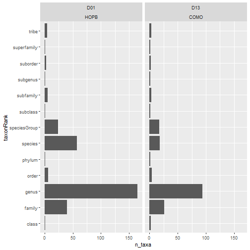
What other visualizations would you plot as an initial exploration of this dataset to determine if it would be sufficient for your science question?

Working with 'long' and 'wide' data

'Reshaping' your data to use as an input to a particular function may require you to consider: do I want 'long' or 'wide' data? Here's a link to a great article from 'the analysis factor' that describes the differences. Our table_observation data.frame is currently in long format, however, many tools used in community ecology analyses, such as functions in the vegan R package, expect wide-format site-by-species inputs.

Below, we create a site-by-species table.

# select only site by species density info and remove duplicate records

table_sample_by_taxon_density_long <- table_observation %>%
  select(sampleID, acceptedTaxonID, inv_dens) %>%
  distinct() %>%
  filter(!is.na(inv_dens))





# pivot to wide format, sum multiple counts per sampleID

table_sample_by_taxon_density_wide <- table_sample_by_taxon_density_long %>%
  tidyr::pivot_wider(id_cols = sampleID, 
                     names_from = acceptedTaxonID,
                     values_from = inv_dens,
                     values_fill = list(inv_dens = 0),
                     values_fn = list(inv_dens = sum)) %>%
  column_to_rownames(var = "sampleID") 



# check col and row sums -- mins should all be > 0

colSums(table_sample_by_taxon_density_wide) %>% min()

## [1] 4

rowSums(table_sample_by_taxon_density_wide) %>% min()

## [1] 32

# Example: use wide format data with functions in vegan

# load library

library(vegan)



# calculate pairwise dissimilarities

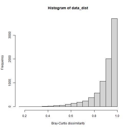
data_dist <- vegdist(table_sample_by_taxon_density_wide, method = "bray")



# view histogram of dissimilarity values in the dataset

hist(data_dist, xlab = "Bray-Curtis dissimilarity")

EXAMPLE 2: North Temperate Lakes (NTL) LTER site benthic macroinvertebrates from the EDI data portal

You can search EDI data holdings at https://portal.edirepository.org/nis/home.jsp. Searching for "benthic macroinvertebrates" will result in data packages from across the LTER network and other NSF funded projects (e.g., data from LTREB and macrosystems projects). For our exmaple, we will use "North Temperate Lakes LTER: Benthic Macroinvertebrates 1981 - current". If you go to the data package landing page and scroll down to the "Code Generation" section, there are buttons to generate scripts to download the dataset from the EDI data portal API. Try clicking the "R" button and running that code in your R session.

• Are these data suitable for your science question?
• Are these data comparable to the NEON benthic macroinvertebrate data set?
• What visualizations would help you determine if this dataset would be useful in your synthesis study?
• What data wrangling steps are needed before you proceed?

Using ecocomDP

Examining the data model for ecocomDP, we see it follows a star-schema with long-format species abundances (or similar) in the observation table. The design pattern includes location, taxon, and other ancillary tables that provide a flexible option to link additional information to the records in the observation, location, and taxon tables. The ecocomDP library for R includes functions to search the EDI and NEON data holdings, read the data into your R session, and functions to work with and plot datasets that are in the ecocomDP format.

Find a NEON ecocomDP dataset

The search_data() function in ecocomDP provides a tool to explore the ecocomDP catalog, which includes datasets from LTER and NEON sites (and others). Using search_data() with no arguments will return the entire catalog. Your search can be constrained by passing a text string (you can use regular expressions) to the text argument. The query will search data package titles, descriptions, and abstracts. Below, we show a couple examples of how to search datasets in the ecocomDP catalog.

# clean out workspace from previous section



#rm(list = ls()) # OPTIONAL - clear out your environment

#gc()            # Uncomment these lines if desired



# search for data sets with periphyton or algae

# regex works!

search_result <- ecocomDP::search_data(text = "periphyt|algae")

View(search_result)



# search for invertebrate data products

search_result <- search_data(text = "invertebrate")

View(search_result)

EXAMPLE 3: Download an ecocomDP formatted NEON macroinvertebrate dataset

You will notice that the ecocomDP version of the NEON macroinvertebrate dataset is listed in the catalog under data package id "neon.ecocomdp.20120.001.001" and "NEON" is indicated as the data source. Here, we will revisit the NEON macroinvertebrate dataset using tools available in the ecocomDP library. When downloading an ecocomDP formatted NEON dataset, the read_data() function in the ecocomDP library uses the same arguments as loadByProduct() from neonUtilities, except now we use the id argument and the ecocomDP id to specify our target data package for download.

# pull NEON aquatic "Macroinvertebrate collection" from the same sites

# and dates as used in the example above.

data_neon_inv <- read_data(
  id = "neon.ecocomdp.20120.001.001",
  site = c("COMO","HOPB"), # NEON sites
  startdate = "2017-01", # start year-month
  enddate = "2019-12", # end year-month
  token = Sys.getenv("NEON_TOKEN"),
  check.size = FALSE)

Now that we have downloaded the data, let's take a look at the ecocomDP data object structure:

# examine the structure of the data object that is returned

data_neon_inv %>% names()

## [1] "id"                "metadata"          "tables"            "validation_issues"

# the data package id

data_neon_inv$id

## [1] "neon.ecocomdp.20120.001.001"

# short list of package summary data

data_neon_inv$metadata$data_package_info

## $data_package_id
## [1] "neon.ecocomdp.20120.001.001.20230803224350"
## 
## $taxonomic_group
## [1] "MACROINVERTEBRATES"
## 
## $orig_NEON_data_product_id
## [1] "DP1.20120.001"
## 
## $NEON_to_ecocomDP_mapping_method
## [1] "neon.ecocomdp.20120.001.001"
## 
## $data_access_method
## [1] "original NEON data accessed using neonUtilities v2.3.0"
## 
## $data_access_date_time
## [1] "2023-08-03 22:43:51 MDT"

# validation issues? None if returns an empty list

data_neon_inv$validation_issues

## list()

# examine the tables

data_neon_inv$tables %>% names()

## [1] "location"              "location_ancillary"    "taxon"                
## [4] "observation"           "observation_ancillary" "dataset_summary"

data_neon_inv$tables$taxon %>% head()

##   taxon_id taxon_rank             taxon_name
## 1   ABLMAL    species   Ablabesmyia mallochi
## 2    ABLSP      genus        Ablabesmyia sp.
## 3   ACASP1   subclass              Acari sp.
## 4   ACEMAC    species Acerpenna macdunnoughi
## 5   ACEPYG    species      Acerpenna pygmaea
## 6    ACESP      genus         Acentrella sp.
##                                      authority_system authority_taxon_id
## 1 Epler 2001, and Maschwitz and Cook 2000; Epler 2001               <NA>
## 2                          Roback 1985 and Epler 2001               <NA>
## 3                               Thorp and Covich 2001               <NA>
## 4                          Morihara & McCafferty 1979               <NA>
## 5           Morihara & McCafferty 1979; Wiersema 2004               <NA>
## 6 Merritt and Cummins 2008; Jacobus & McCafferty 2006               <NA>

data_neon_inv$tables$observation %>% head()

##   observation_id                event_id                                 package_id
## 1          obs_1 COMO.20170803.KICKNET.1 neon.ecocomdp.20120.001.001.20230803224350
## 2          obs_2 COMO.20170803.KICKNET.1 neon.ecocomdp.20120.001.001.20230803224350
## 3          obs_3 COMO.20170803.KICKNET.1 neon.ecocomdp.20120.001.001.20230803224350
## 4          obs_4 COMO.20170803.KICKNET.1 neon.ecocomdp.20120.001.001.20230803224350
## 5          obs_5 COMO.20170803.KICKNET.1 neon.ecocomdp.20120.001.001.20230803224350
## 6          obs_6 COMO.20170803.KICKNET.1 neon.ecocomdp.20120.001.001.20230803224350
##      location_id            datetime taxon_id variable_name value                   unit
## 1 COMO.AOS.reach 2017-08-03 15:29:00   ARRSP2       density    12 count per square meter
## 2 COMO.AOS.reach 2017-08-03 15:29:00   BILALG       density   424 count per square meter
## 3 COMO.AOS.reach 2017-08-03 15:29:00    BRISP       density     8 count per square meter
## 4 COMO.AOS.reach 2017-08-03 15:29:00  CERSP10       density     8 count per square meter
## 5 COMO.AOS.reach 2017-08-03 15:29:00  CHESP17       density     8 count per square meter
## 6 COMO.AOS.reach 2017-08-03 15:29:00   CHISP6       density     8 count per square meter

Notice that the records in the observation table are reported as densities standardize per unit effort (i.e., area sampled). All of the data wrangling that we needed to do in the section above is coded into the mapping code used in ecocomDP for this NEON data product. It is important to note that this mapping is a work in progress for ecocomDP datasets. If you have recommendations to improve a dataset mapping to the ecocomDP format, an alternative mapping, or a new dataset that you would like to see mapped to the ecocomDP format, feel free to make a new issue on the ecocomDP GitHub repo.

Built-in tools for quick data vis

The ecocomDP package offers some useful data visualization tools.

# Explore the spatial and temporal coverage 

# of the dataset

data_neon_inv %>% plot_sample_space_time()

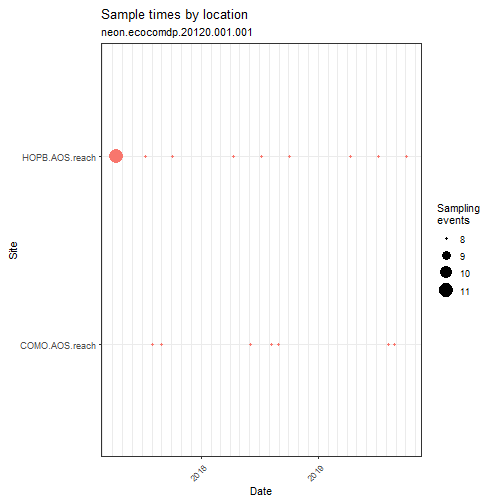
# As noted above, this plot shows replicate "event_id's" can occur

# at the same time at the same site, indicating these are replicate

# observations or samples. 


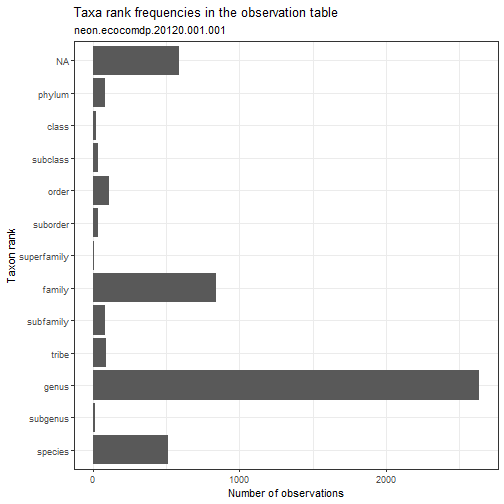
# Explore the taxonomic resolution in the dataset. 

# What is the most common taxonomic resolution (rank) 

# for macroinvertebrate identifications in this dataset?

data_neon_inv %>% plot_taxa_rank()

Manipulating ecocomDP data objects

The flatten_data() function will properly flatten and merge all the tables in an ecocomDP dataset, including any hierarchical spatial data in the location table. The flat view can be useful for examining how ancillary data can provide context for observations and provide options for grouping data in plots.

# combine all core and ancillary tables into one flat table and explore

# NOTE: we add the id so we can stack with other datasets

flat_neon_inv <- data_neon_inv %>% 
  flatten_data() %>%
  mutate(id = data_neon_inv$id) 

View(flat_neon_inv)



# note that event_id maps to a sample ID in the dataset

# we can tell because multiple event_id's can share a site and date


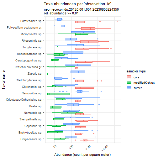
# compare taxa and abundances across sampler types

flat_neon_inv %>% 
  plot_taxa_abund(
    trans = "log10",
    min_relative_abundance = 0.01,
    color_var = "samplerType")

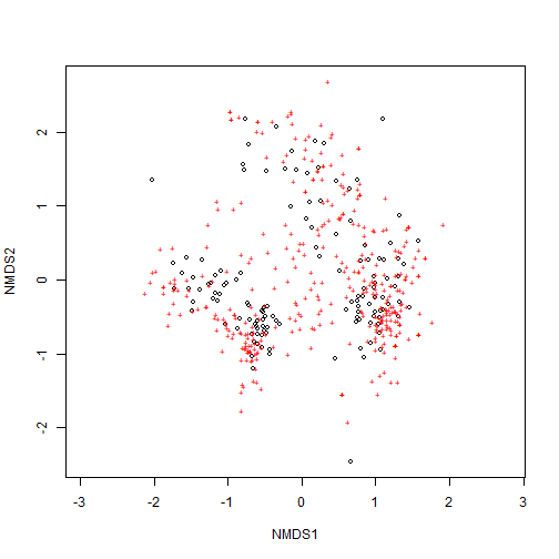
The ecocomDP format is also easy to pivot to wide format for input to commonly used analyses, such as the ordination functions in the vegan package for R.

# make wide, event_id by taxon_id

wide_neon_inv <- data_neon_inv$tables$observation %>%
  pivot_wider(
    id_cols = event_id,
    names_from = taxon_id,
    values_from = value,
    values_fill = 0) %>%
  tibble::column_to_rownames("event_id")



# make sure now rows or columns sum to 0

rowSums(wide_neon_inv) %>% min()

## [1] 32

colSums(wide_neon_inv) %>% min()  

## [1] 4

# load vegan library for ordination analysis

library(vegan)



# create ordination using metaMDS

my_nmds_result <- wide_neon_inv %>% metaMDS()

## Square root transformation
## Wisconsin double standardization
## Run 0 stress 0.1977579 
## Run 1 stress 0.2153616 
## Run 2 stress 0.2298491 
## Run 3 stress 0.2359556 
## Run 4 stress 0.2233196 
## Run 5 stress 0.2090286 
## Run 6 stress 0.2466269 
## Run 7 stress 0.1990968 
## Run 8 stress 0.2382048 
## Run 9 stress 0.2305114 
## Run 10 stress 0.1960912 
## ... New best solution
## ... Procrustes: rmse 0.02992648  max resid 0.3227259 
## Run 11 stress 0.2499347 
## Run 12 stress 0.2088631 
## Run 13 stress 0.1952428 
## ... New best solution
## ... Procrustes: rmse 0.007730752  max resid 0.08461392 
## Run 14 stress 0.2098515 
## Run 15 stress 0.2158888 
## Run 16 stress 0.1961931 
## Run 17 stress 0.2492565 
## Run 18 stress 0.2514713 
## Run 19 stress 0.2233795 
## Run 20 stress 0.2134943 
## *** Best solution was not repeated -- monoMDS stopping criteria:
##     17: stress ratio > sratmax
##      3: scale factor of the gradient < sfgrmin

# ordination stress

my_nmds_result$stress

## [1] 0.1952428

# plot ordination

ordiplot(my_nmds_result)

EXAMPLE 4: Compare NEON and LTER ecocomDP datasets

Let's compare the full NEON benthic macroinvertebrate dataset pusblished in the 2022 Data Release (RELEASE-2022: https://doi.org/10.48443/gn8x-k322) to an LTER benthic macroinvertebrate dataset from the North Temperate Lates (NTL) LTER site.

The full NEON macroinvertebrate dataset from RELEASE-2022 can be downloaded into the ecocomDP format using the code below; however, I have already downloaded this dataset and saved it to the CyVerse Data Store for this workshop (so don't run this code chunk).

# pull NEON aquatic "Macroinvertebrate collection" for all locations and times

# in the 2022 Data Release



# This could take up to 10 mins

data_neon_inv_allsites <- read_data(

  id = "neon.ecocomdp.20120.001.001",

  token = Sys.getenv("NEON_TOKEN"),

  release = "RELEASE-2022",

  check.size = FALSE)

The above download has been saved in the CyVerse Data Store for easy access from the VICE RStudio app. There are three options for accessing the file:

1. If you are using the RStudio VICE app:

   data_neon_inv_allsites <- readRDS("../rstudio/work/home/shared/NEON/ESA2022/macroinverts_neon.ecocomdp.20120.001.001_release2022.RDS")

2. If you are not running an in instance of RStudio that has the CyVerse Data Store mounted, you can access the data here via a static URL:

   data_neon_inv_allsites <- readRDS( file = gzcon(url("https://data.cyverse.org/dav-anon/iplant/projects/NEON/ESA2022/macroinverts_neon.ecocomdp.20120.001.001_release2022.RDS")))

3. You can download the file from your web browser from the CyVerse DE web UI. To navigate to the dataset using the CyVerse Discovery Environment webUI, go to the Data Store icon on in the left menu, choose "Community Data" in the dropdown menu, and then navigate to "NEON > ESA2022 > macroinverts_neon.ecocomdp.20120.001.001_release2002.RDS". Here you can download the dataset and work with it locally on your machine.

Next, we will flatten the dataset:

flat_neon_inv_allsites <- data_neon_inv_allsites %>% flatten_data()

Now we will see if we can find a comparable LTER benthic macroinvertebrate dataset. In the search_result data.frame, the dataset with id "edi.290.2" titled "North Temperate Lakes LTER: Benthic Macroinvertebrates 1981 - current (Reformatted to the ecocomDP Design Pattern)" seems like a good candidate (Note: this is derived from the dataset used in "Example 2" above). Let's download and flatten this dataset.

# pull data for NTL aquatic macroinvertebrates to compate

data_ntl_inv <- read_data(id = "edi.290.2")



# flatten the dataset

flat_ntl_inv <- data_ntl_inv %>% flatten_data()



View(flat_ntl_inv)

Next, we can stack the NEON and the North Temperate Lakes (NTL) LTER benthic macroinvertebrate datasets and make some plots to explore if these two datasets are comparable. Many of the built-in ecocomDP plotting functions will work with the stacked datasets because they both have the same required core ecocomDP variables. However, the ancillary variabiles from each dataset will be different, and these fields will not be useful in the stacked dataset.

# The NEON dataset is pretty extensive, including streams and lakes. Let's

# look at what kind of ancillary data are included that might be useful

# for filtering the dataset:

flat_neon_inv_allsites %>% names()

##  [1] "observation_id"              "event_id"                    "datetime"                   
##  [4] "variable_name"               "value"                       "unit"                       
##  [7] "estimatedTotalCount"         "individualCount"             "subsamplePercent"           
## [10] "laboratoryName"              "publicationDate"             "release"                    
## [13] "benthicArea"                 "neon_event_id"               "habitatType"                
## [16] "samplerType"                 "substratumSizeClass"         "remarks"                    
## [19] "ponarDepth"                  "snagLength"                  "snagDiameter"               
## [22] "location_id"                 "location_name"               "siteID"                     
## [25] "latitude"                    "longitude"                   "elevation"                  
## [28] "domainID"                    "aquaticSiteType"             "taxon_id"                   
## [31] "taxon_rank"                  "taxon_name"                  "authority_system"           
## [34] "package_id"                  "original_package_id"         "length_of_survey_years"     
## [37] "number_of_years_sampled"     "std_dev_interval_betw_years" "max_num_taxa"

# what kind of aquaticSiteTypes are in the data?

flat_neon_inv_allsites$aquaticSiteType %>% unique()

## [1] "stream" "lake"   "river"

# Let's filter the NEON dataset to aquaticSitetypes that are "lake", and

# only include sites in Domain 5, because those sites are relatively close 

# to the NTL LTER site (in Wisconsin)

flat_neon_inv_d05 <- flat_neon_inv_allsites %>%
  filter(aquaticSiteType == "lake",
         domainID == "D05")



# stack two datasets

stacked_inv <- bind_rows(
  flat_neon_inv_d05,
  flat_ntl_inv) %>% 
  as.data.frame()



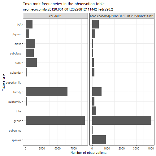
# compare taxon ranks used in the two data sets

stacked_inv %>% 
  plot_taxa_rank(
    facet_var = "package_id",
    facet_scales = "free_x")

# compare spatial and temporal replication

# updates are planned for this plotting function to allow 

# additional aesthetic mappings and faceting

stacked_inv %>%
  plot_sample_space_time()

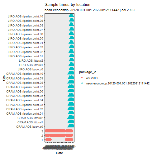Notice that the NTL sites have a much longer time series and the NEON data add a good amount of spatial replication.

# plot on a US Map



# NOTE: for this to work, you may need to install some dependencies that 

# are not automatically installed with the ecocomDP package.

#

# install.packages(c("ggrepel", "usmap", "maptools", 

#                    "rgdal", "ecocomDP", "neonUtilities"), dependencies=TRUE)



stacked_inv %>%

  plot_sites()



# Figure not shown


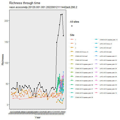
# explore richness through time

stacked_inv %>% 
  plot_taxa_diversity(time_window_size = "year") 

# compare taxa and abundances

stacked_inv %>% 
  plot_taxa_occur_freq(
    facet_var = "package_id")

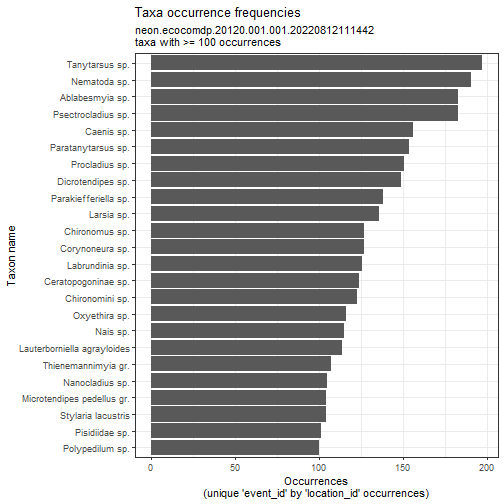
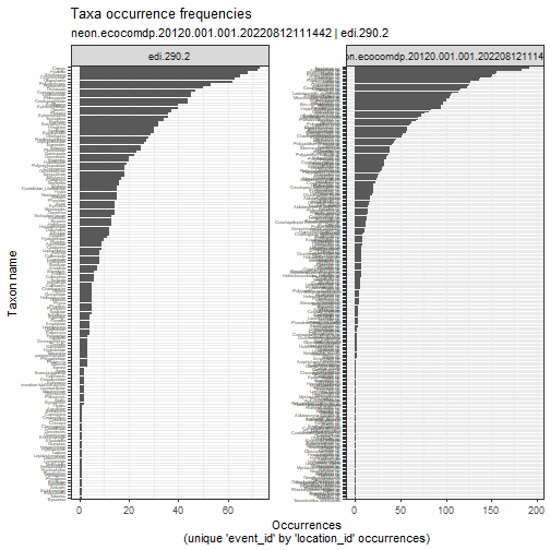To actually see the top taxa in each dataset, we need to plot them separately.

# Plot common NEON taxa abundances

# you can set the min_occurrence argument to have a reasonable cutoff based 

# on the plot above

flat_neon_inv_d05 %>% 
  plot_taxa_occur_freq(min_occurrence = 100)

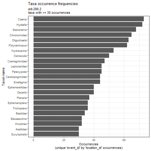
# Plot common NTL taxa abundances

flat_ntl_inv %>% 
  plot_taxa_occur_freq(min_occurrence = 30)

Moving forward with synthesis

• Would you be able to use these two datasets in a synthesis project?
• What additional data wrangling would you need to do to combine these data in an analysis?
• Are there other datasets in ecocomDP that you could add to a synthesis project?