Modeling phenology with the R package phenor

This tutorial focuses on aggregating and combining various climate and phenology data sources for modeling purposes using the phenor R package. This tutorial explains the various data sources and in particular phenocam data, the structure of the formatted data and the final modelling procedures using various phenology models.

This tutorial has three parts:

1. Introductions to the relevant R packages
2. Aggregating & format the data
3. Model phenology

Due to the the large size of the data involved, we will learn how to obtain research quality data in the aggregating data steps but we will use pre-subsetted data sets for the modeling. The pre-subsetted sets can be downloaded at the end of each section or directly accessed during the modeling section.

The R packages

phenor

The phenor R package is a phenology modeling framework in R. The framework leverages measurements of vegetation phenology from four common phenology observation datasets combined with (global) retrospective and projected climate data. Currently, the package focuses on North America and Europe and relies heavily on Daymet and E-OBS climate data for underlying climate driver data in model optimization. The package supports global gridded CMIP5 forecasts for RCP4.5 and RCP8.5 climate change scenarios using the NASA Earth Exchange global downscaled daily projections.

Phenological model calibration and validation data are derived from four main sources:

• the transition dates derived from PhenoCam time series and included in this package.
• the MODIS MCD12Q2 phenology product using the MODISTools R package
• the Pan European Phenology Project (PEP725)
• the USA National Phenological Network (USA-NPN).

phenocamr

We will also use the the phenocamr package in the processing of data provided through the PhenoCam API and past data releases. Although the uses of standard product releases is encouraged in some instances you might want more control over the data processing and the transition date products generated. phenocamr provides this flexibility.

Get PhenoCam Data

In this tutorial, you are going to download PhenoCam time series, extract transition dates and combine the derived spring phenology data, Daymet data, to calibrate a spring phenology model. Finally, you make projections for the end of the century under an RCP8.5 CMIP5 model scenario.

The PhenoCam Network includes data from around the globe (map.) However, there are other data sources that may be of interest including the Pan European Phenology Project (PEP725). For more on accessing data from the PEP725, please see the final section of this tutorial.

First, we need to set up our R environment.

# uncomment for install
# install.packages("devtools")
# install_github("khufkens/phenor")
# install.packages("phenocamr")
# install.packages("maps")

library("phenocamr")
library("phenor")
library("maps")
library("raster")

To download phenology data from the PhenoCam network use the download_phenocam() function from the phenocamr package. This function allows you to download site based data and process it according to a standardized methodology. A full description of the methodology is provided in Scientific Data: Tracking vegetation phenology across diverse North American biomes using PhenoCam imagery (Richardson et al. 2018).

The code below downloads all time series for deciduous broadleaf data at the Bartlett Experimental Forest (bartlettir) PhenoCam site and estimate the phenophases (spring & autumn). For a detailed description of the download procedure consult the phenocamr R package documentation.

# download the three day time series for deciduous broadleaf data at the 
# Bartlett site and will estimate the phenophases (spring + autumn). 

phenocamr::download_phenocam(
  frequency = 3,
  veg_type = "DB",
  roi_id = 1000,
  site = "bartlettir",
  phenophase = TRUE,
  out_dir = "."
  )

## Downloading: bartlettir_DB_1000_3day.csv

## -- Flagging outliers!

## -- Smoothing time series!

## -- Estimating transition dates!

Using the code (out_dir = ".") causes the downloaded data, both the 3-day time series and the calculated transition dates, to be stored in your current working directory. You can change that is you want to save it elsewhere. You will get feedback on the processing steps completed.

We can now load this data; both the time series and the transition files.

# load the time series data
df <- read.table("bartlettir_DB_1000_3day.csv", header = TRUE, sep = ",")

# read in the transition date file
td <- read.table("bartlettir_DB_1000_3day_transition_dates.csv",
                 header = TRUE,
                 sep = ",")

Threshold values

Now let's plot the data to see what we are working with. But first, let's subset the transition date (td) for each year when 25% of the greenness amplitude (of the 90^th^) percentile is reached (threshold_25).

# select the rising (spring dates) for 25% threshold of Gcc 90
td <- td[td$direction == "rising" & td$gcc_value == "gcc_90",]

# create a simple line graph of the smooth Green Chromatic Coordinate (Gcc)
# and add points for transition dates
plot(as.Date(df$date), df$smooth_gcc_90, type = "l", xlab = "Date",
     ylab = "Gcc (90th percentile)")
points(x = as.Date(td$transition_25, origin = "1970-01-01"),
       y = td$threshold_25,
       pch = 19,
       col = "red")

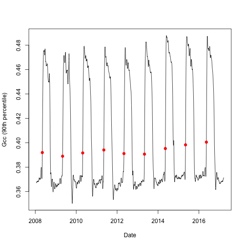
Now we can se the transition date for each year of interest and the annual patterns of the Gcc.

However, if you want more control over the parameters used during processing, you can run through the three default processing steps as implemented in download_phenocam() and set parameters manually.

Of particular interest is the option to specify your own threshold used in determining transition dates. In the example below, we will set the upper threshold value to 80% of the amplitude (or 0.8). We will visualize the data as above, showing the newly found transition dates along the Gcc curve.

# the first step in phenocam processing is flagging of the outliers
# on the file you visualized in the previous step
detect_outliers("bartlettir_DB_1000_3day.csv",
                out_dir = ".")

# the second step involves smoothing the data using an optimization approach
# we force the procedure as it will be skipped if smoothed data is already
# available
smooth_ts("bartlettir_DB_1000_3day.csv",
          out_dir = ".",
          force = TRUE)

# the third and final step is the generation of phenological transition dates
td <- phenophases("bartlettir_DB_1000_3day.csv",
            internal = TRUE,
            upper_thresh = 0.8)

Now we have manually set the parameters that were default for our first plot. Note, that here is also a lower and a middle threshold parameter, the order matters so always use the relevant parameter (for parameters, check transition_dates())

Now we can again plot the annual pattern with the transition dates.

# split out the rising (spring) component for Gcc 90th
td <- td$rising[td$rising$gcc_value == "gcc_90",]

# we can now visualize the upper threshold
plot(as.Date(df$date), df$smooth_gcc_90, type = "l",
     xlab = "Date",
     ylab = "Gcc (90th percentile)")
points(x = as.Date(td$transition_80, origin = "1970-01-01"),
       y = td$threshold_80,
       pch = 19,
       col = "red")

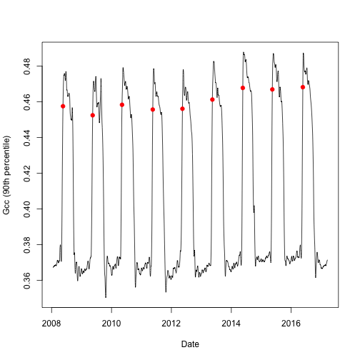
With the above examples you can get a feeling of how to manually re-process PhenoCam time series.

Phenocam Subsetted Data Set

To allow our models to run in a timely manner, we will use the subsetted data that is included with the phenor packages for the modeling portion of this tutorial. All deciduous broadleaf forest data in the PhenoCam V1.0 have been processed using the above settings. This data set is called phenocam_DB.

Alternatively, you can download a curated dataset from the ORNL DAAC, as fully described in Scientific Data: Tracking vegetation phenology across diverse North American biomes using PhenoCam imagery (Richardson et al. 2018). A limited copy, including only time series and transition dates, is also mirrored as a github repo (500 mb).

Get Climate Data

In order to calibrate phenology models, additional climate data is required. Some of this data is dynamically queried during the formatting of the data. Alternatively, we can get climate data from another source, like the Coupled Model Intercomparison Project (CMIP5). The forecast CMIP5 data is gridded data which is too large to process dynamically. In order to use the CMIP5 data to make phenology projections the data needs to be downloaded one year at a time, and subset where possible to reduce file sizes. Below you find the instructions to download the 2090 CMIP5 data for the RCP8.5 scenario of the MIROC5 model. The data will be stored in the R temporary directory for later use. Please note that this is a large file (> 4 GB).

# download source cmip5 data into your temporary directory
# please note this is a large download: >4GB! 
phenor::download_cmip5(
  year = 2090,
  path = tempdir(),
  model = "MIROC5",
  scenario = "rcp85"
  )

phenor::download_cmip5(
  year = 2010,
  path = tempdir(),
  model = "MIROC5",
  scenario = "rcp85"
  )

Format Phenology & Climate Data

If both phenology and climate data are available you can aggregate and format the data for modeling purposes. All functions in the phenor package with a format_ prefix serve this purpose, although some might lack phenology validation data.

You can format phenocam data using the format_phenocam() function, which requires you to provide the correct path to phenocam transition date files, like those we downloaded above). This function will match the transition dates from PhenoCam data with the appropriate Daymet data (dynamically).

In the next code chunk, we will format the phenocam transition date data (in your working directory, ".") correctly. Then we will specify the direction of the curve to be considered and setting the Gcc percentile, threshold and temporal offset.

# Format the phenocam transition date data 
# Specify the direction of the curve 
# Specify the gcc percentile, threshold and the temporal offset

phenocam_data <- phenor::format_phenocam(
  path = ".",
  direction = "rising",
  gcc_value = "gcc_90",
  threshold = 50,
  offset = 264,
  internal = TRUE
  )

## Processing 1 sites
## 

|
| | 0% |
|==================================================================================| 100%

# When internal = TRUE, the data will be returned to the R
# workspace, otherwise the data will be saved to disk.

# view data structure
str(phenocam_data)

## List of 1
##  $ bartlettir:List of 13
##   ..$ site            : chr "bartlettir"
##   ..$ location        : num [1:2] 44.1 -71.3
##   ..$ doy             : int [1:365] -102 -101 -100 -99 -98 -97 -96 -95 -94 -93 ...
##   ..$ ltm             : num [1:365] 13.5 14.1 13.6 13 11.9 ...
##   ..$ transition_dates: num [1:9] 133 129 122 133 130 128 136 130 138
##   ..$ year            : num [1:9] 2008 2009 2010 2011 2012 ...
##   ..$ Ti              : num [1:365, 1:9] 16 17.2 16.8 15.5 16.2 ...
##   ..$ Tmini           : num [1:365, 1:9] 7 10 10.5 7.5 6.5 11 16 14.5 7.5 3 ...
##   ..$ Tmaxi           : num [1:365, 1:9] 25 24.5 23 23.5 26 29 28.5 24 20 18 ...
##   ..$ Li              : num [1:365, 1:9] 11.9 11.9 11.8 11.8 11.7 ...
##   ..$ Pi              : num [1:365, 1:9] 0 0 0 0 0 0 5 6 0 0 ...
##   ..$ VPDi            : num [1:365, 1:9] 1000 1240 1280 1040 960 1320 1800 1640 1040 760 ...
##   ..$ georeferencing  : NULL
##  - attr(*, "class")= chr "phenor_time_series_data"

As you can see, this formats a nested list of data. This nested list is consistent across all format_ functions.

Finally, when making projections for the coming century you can use the format_cmip5() function. This function does not rely on phenology data but creates a consistent data structure so models can easily use this data. In addition, there is the option to constrain the data, which is global, spatially with an extent parameter. The extent is a vector with coordinates defining the region of interest defined as xmin, xmax, ymin, ymax in latitude and longitude.

This code has a large download size, we do not show the output of this code.

# format the cmip5 data
cmip5_2090 <- phenor::format_cmip5(
  path = tempdir(), 
  year = 2090,
  offset = 264,
  model = "MIROC5",
  scenario = "rcp85",
  extent = c(-95, -65, 24, 50),
  internal = FALSE
  )

cmip5_2010 <- phenor::format_cmip5(
  path = tempdir(), 
  year = 2010,
  offset = 264,
  model = "MIROC5",
  scenario = "rcp85",
  extent = c(-95, -65, 24, 50),
  internal = FALSE
  )

Climate Training Dataset

Given the large size of the climate projection data above, we will use subsetted and formatted training dataset. In that section of the tutorial, we will directly read the data into R.

Alternatively, you can download it here as a zip file (128 MB) or obtain the data by cloning the GitHub repository,

git clone https://github.com/khufkens/phenocamr_phenor_demo.git

Now that we have the needed phenology and climate projection data, we can create our model.

Phenology Model Parameterization

Gathering all this data serves as input to a model calibration routine. This routine tweaks parameters in the model specification in order to best fit the response to the available phenology data using the colocated climate driver data.

The default optimization method uses Simulated Annealing to find optimal parameter sets. Ideally the routine is run for >10K iterations (longer for complex models). When the procedure ends, by default, a plot of the modeled ~ measured data is provided in addition to model fit statistics. This gives you quick feedback on model accuracy.

For a full list of all models included and their model structure, please refer to the package documentation and Hufkens et al. 2018. An integrated phenology modelling framework in R: Phenology modelling with phenor.

For the phenology data, we'll used the example data that comes with phenor. This will allow our models to run faster than if we used all the data we downloaded in the second part of this tutorial. phencam_DB includes a subset of the deciduous broadleaf forest data in the PhenoCam V1.0. This has all been processed using the settings we used above.

# load example data
data("phenocam_DB")

# Calibrate a simple Thermal Time (TT) model using simulated annealing
# for both the phenocam and PEP725 data. This routine might take some
# time to execute.
phenocam_par <- model_calibration(
  model = "TT",
  data = phenocam_DB,
  method = "GenSA",
  control = list(max.call = 4000),
  par_ranges = sprintf("%s/extdata/parameter_ranges.csv", path.package("phenor")),
  plot = TRUE)

## 
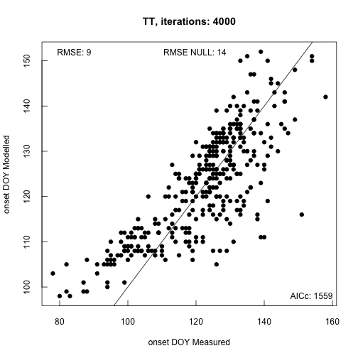
## Call:
## stats::lm(formula = data$transition_dates ~ out)
## 
## Residuals:
##     Min      1Q  Median      3Q     Max 
## -24.311  -5.321  -1.247   4.821  35.776 
## 
## Coefficients:
##              Estimate Std. Error t value Pr(>|t|)    
## (Intercept) 0.0009523  4.9037867    0.00        1    
## out         0.9933004  0.0397814   24.97   <2e-16 ***
## ---
## Signif. codes:  0 '***' 0.001 '**' 0.01 '*' 0.05 '.' 0.1 ' ' 1
## 
## Residual standard error: 8.737 on 356 degrees of freedom
## Multiple R-squared:  0.6365,	Adjusted R-squared:  0.6355 
## F-statistic: 623.4 on 1 and 356 DF,  p-value: < 2.2e-16

# you can specify or alter the parameter ranges as located in
# copy this file and use the par_ranges parameter to use your custom version
print(sprintf("%s/extdata/parameter_ranges.csv", path.package("phenor")))

## [1] "/Library/Frameworks/R.framework/Versions/3.6/Resources/library/phenor/extdata/parameter_ranges.csv"

We can list the parameters by looking at one of the nested list items (par).

# only list the TT model parameters, ignore other
# ancillary fields
print(phenocam_par$par)

## [1] 176.35246  -4.39729 549.56298

Phenology Model Predictions

To finally evaluate how these results would change phenology by the end of the century we use the formatted CMIP5 data to estimate_phenology() with those given drivers.

We will use demo CMIP5 data, instead of the data we downloaded earlier, so that our model comes processes faster.

# download the cmip5 files from the demo repository
download.file("https://github.com/khufkens/phenocamr_phenor_demo/raw/master/data/phenor_cmip5_data_MIROC5_2090_rcp85.rds",
              "phenor_cmip5_data_MIROC5_2090_rcp85.rds")

download.file("https://github.com/khufkens/phenocamr_phenor_demo/raw/master/data/phenor_cmip5_data_MIROC5_2010_rcp85.rds",
              "phenor_cmip5_data_MIROC5_2010_rcp85.rds")

# read in cmip5 data
cmip5_2090 <- readRDS("phenor_cmip5_data_MIROC5_2090_rcp85.rds")
cmip5_2010 <- readRDS("phenor_cmip5_data_MIROC5_2010_rcp85.rds")

Now that we have both the phenocam data and the climate date we want run our model projection.

# project results forward to 2090 using the phenocam parameters
cmip5_projection_2090 <- phenor::estimate_phenology(
  par = phenocam_par$par, # provide parameters
  data = cmip5_2090, # provide data
  model = "TT" # make sure to use the same model !
)

# project results forward to 2010 using the phenocam parameters
cmip5_projection_2010 <- phenor::estimate_phenology(
  par = phenocam_par$par, # provide parameters
  data = cmip5_2010, # provide data
  model = "TT" # make sure to use the same model !
)

If data are gridded data, the output will automatically be formatted as raster data, which can be plotted using the raster package as a map.

Let's view our model.

# plot the gridded results and overlay
# a world map outline
par(oma = c(0,0,0,0))
raster::plot(cmip5_projection_2090, main = "DOY")
maps::map("world", add = TRUE)

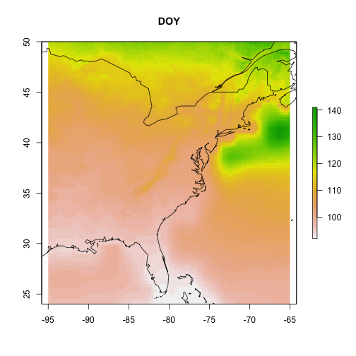
Maybe more intersting is showing the difference between the start (2010) and the end (2090) of the century.

# plot the gridded results and overlay
# a world map outline for reference
par(oma = c(0,0,0,0))
raster::plot(cmip5_projection_2010 - cmip5_projection_2090,
             main = expression(Delta * "DOY"))
maps::map("world", add = TRUE)

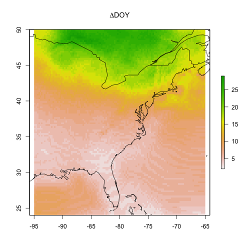
What can you take away from these model visualizations?

PEP725 data

To get phenocam data for Europe. you will likely want to use the Pan European Phenology Project (PEP725). This section teaching you how to access PEP725 data.

PEP725 Log In

Downloading data from the PEP725 network using phenor is more elaborate as it requires a login on the PEP725 website before you can access any data.

In order to move forward with this tutorial, create a login on the PEP725 website and save your login details in a plain text file (.txt) containing your email address and password on the first and second line, respectively. Name this file appropriately (e.g., pep725_credentials.txt.)

PEP725 Data Availability

To download PEP725 data you need to find out which data are available. You can either consult the data portal of the website, or use the check_pep725_species() function. This function allows you to either list all species in the dataset, or search by (partial) matches on the species names.

# to list all species use
species_list <- phenor::check_pep725_species(list = TRUE)

## Warning in xml2::read_html(data_selection): restarting interrupted promise evaluation

## Warning in xml2::read_html(data_selection): internal error -3 in R_decompress1

## Error in xml2::read_html(data_selection): lazy-load database '/Library/Frameworks/R.framework/Versions/3.6/Resources/library/xml2/R/xml2.rdb' is corrupt

# to search only for Quercus (oak) use
quercus_nr <- phenor::check_pep725_species(species = "quercus")

## Warning in xml2::read_html(data_selection): restarting interrupted promise evaluation

## Warning in xml2::read_html(data_selection): internal error -3 in R_decompress1

## Error in xml2::read_html(data_selection): lazy-load database '/Library/Frameworks/R.framework/Versions/3.6/Resources/library/xml2/R/xml2.rdb' is corrupt

# return results
head(species_list)

## Error in head(species_list): object 'species_list' not found

head(quercus_nr)

## Error in head(quercus_nr): object 'quercus_nr' not found

A query for Quercus returns a species ID number of 111. Once you have established the required species number you can move forward and download the species data.

phenor::download_pep725(
  credentials = "~/pep725_credentials.txt",
  species = 111,
  path = ".",
  internal = FALSE
  )

The data use policy does not allow to distribute data so this will conclude the tutorial portion on downloading PEP725 observational data. However, the use of the formatting functions required in phenor is consistent and the example using PhenoCam data, above, should make you confident in processing data from the PEP725 database once downloaded.

PEP Climate Data

For the formatting of the PEP725 data, no automated routine is provided due to the size of the download and policy of the E-OBS dataset. Register and download the E-OBS data for the 0.25 degree regular grid for the best estimates of TG, TN, TX, RR, PP (0.5 degree data is supported but not recommended).

Format PEP Climate Data

Similarly, the PEP725 data have a dedicated formatting function in the phenor package, format_pep725(). However, it will use the previously downloaded E-OBS data to provided the required climate data for the downloaded PEP725 data (both file directories are requested). In addition, you need to specify which BBCH-scale value you would like to see included in the final formatted dataset.

# provisional query, code not run due to download / login requirements
pep725_data <- phenor::format_pep725(
  pep_path = ".",
  eobs_path = "/your/eobs/path/",
  bbch = "11",
  offset = 264,
  count = 60,
  resolution = 0.25
  )