Workshop
Spatio-Temporal Workshop
NEON & Data Carpentry
-
This two day workshop, taught at the USGS National Training Center at the Federal Center in Denver, CO on April 12-13, 2016, will cover how to work with spatio-temporal data in R.
Software
R & RStudio
To participant in this workshop, you will need a laptop with the most current version of R, and, preferably, RStudio loaded on your computer. You will also need the bash shell installed
If you already have these installed on your laptop, please be sure that you are running the most current version of RStudio, R and all packages that we'll be using in the workshop (listed below).
For details on installing RStudio in Mac, PC, or Linux operating systems, please see the Additional Set Up Instructions section at the bottom of this page.
Bash shell
You will need bash shell to complete this workshop. If you use a Mac, this is the default shell ("Terminal") on your computer. If you use a PC or Linux operating system you may need to install it. For complete installation instructions, please see the Additional Set Up Instructions section below.
Download Data
To be prepared for this workshop, please download & unzip the following files in advance:
[[nid:6355]] [[nid:6345]] [[nid:6351]]
Optional: you can download the global boundary files below if you wish to follow along with the data management demonstration on Coordinate Reference Systems.
-
Download "land" - Natural Earth Global Continent Boundary Layer
-
Download all Graticules - Natural Earth Global Graticules Layer
So that your code will mirror that of the instructors, your R working directory should be set to a parent directory data that contains all of the above data files (unzipped). For complete directions, please see the Additional Set Up Instructions section below.
Install R Packages
You can chose to install each library individually if you already have some installed.
-
raster:
install.packages("raster") -
rasterVis:
install.packages("rasterVis") -
ggplot2:
install.packages("ggplot2") -
sp:
install.packages("sp") -
rgeos
install.packages("rgeos") -
rgdal (windows):
install.packages("rgdal") -
rgdal (mac):
install.packages("rgdal",configure.args="--with-proj-include=/Library/Frameworks/PROJ.framework/unix/include --with-gdal-config=/Library/Frameworks/GDAL.framework/unix/bin/gdal-config --with-proj-lib=/Library/Frameworks/PROJ.framework/unix/lib")
Optional installation If you want to work through the metadata lesson which includes a section on the Ecological Metadata Language (EML), please install the following:
-
devtools:
install.packages("devtools") -
eml
install_github("ropensci/EML", build=FALSE, dependencies=c("DEPENDS", "IMPORTS"))NOTE: You have to run the devtools librarylibrary(devtools)first, and theninstall_githubwill work the EML package is under development which is why the install occurs from GitHub and not can!
Update R Packages
In RStudio, you can go to Tools --> Check for package updates to update already installed libraries on your computer! Or, you can use update.packages() to update all packages that are installed in R automatically.
Workshop Instructors
- Leah Wasser; @leahawasser; Supervising Scientist, NEON
- Megan A. Jones; @meganahjones; Staff Scientists/Science Educator, NEON
- Natalie Robinson; Staff Scientist, NEON
Please get in touch with the instructors prior to the workshop with any questions.
Twitter?
Please tweet @NEON_sci and with the #WorkWithData hashtag during the workshop.
Schedule
Please note that the schedule listed below may change depending upon the pace of the workshop!
Day One
| Time | Topic |
|---|---|
| 8:00 | Please come early if you have any setup or installation problems |
| 9:00 | Geospatial Data Management - Intro to Geospatial Concepts |
| 10:30 | --------- BREAK --------- |
| 10:45 | Data Management: Coordinate Reference Systems |
| 12:00 | --------- Lunch --------- |
| 1:00 | Vector Data in R |
| 2:30 | --------- BREAK --------- |
| 2:45 | Vector Data in R, continued |
| 4:15 | Wrap-Up Day 1 |
Day Two
| Time | Topic |
|---|---|
| 9:00 | Questions From Day One |
| 9:15 | Getting Started with Raster Data in R |
| 10:30 | --------- BREAK --------- |
| 10:45 | Getting Started with Raster Data in R, continued |
| 12:00 | --------- Lunch --------- |
| 1:00 | Multi-band Raster & Raster Time Series Data in R |
| 2:30 | --------- BREAK --------- |
| 2:45 | Multi-band Raster & Raster Time Series Data in R, continued |
| 4:15 | Wrap-Up Day Two! |
Additional Set Up Resources
[[nid:6408]]
[[nid:6512]]
GDAL installation for MAC
You may need to install GDAL in order for rgdal to work properly. Click here to watch a video on installing gdal using homebrew on your Mac. Or, you can visit this link to install GDAL 1.11 complete.
Day One
| Time | Topic |
|---|---|
| 8:00 | Please come early if you have any setup or installation problems |
| 9:00 | Geospatial Data Management - Intro to Geospatial Concepts |
| Answer a Spatio-temporal Research Question with Data - Where to Start? | |
| Data Management: Spatial Data Formats | |
| Data about Data -- Intro to Metadata Formats & Structure | |
| 10:30 | --------- BREAK --------- |
| 10:45 | Data Management: Coordinate Reference Systems |
| 12:00 - 1:00 | --------- Lunch --------- |
| 1:00 | Vector Data in R |
| Open and Plot Shapefiles in R - Getting Started with Point, Line and Polygon Vector Data | |
| Explore Shapefile Attributes & Plot Shapefile Objects by Attribute Value in R | |
| Plot Multiple Shapefiles and Create Custom Legends in Base Plot in R | |
| 2:30 | --------- BREAK --------- |
| 2:45 | Vector Data in R, continued |
| When Vector Data Don't Line Up - Handling Spatial Projection & CRS in R | |
| Convert from .csv to a Shapefile in R | |
| 4:15 | Wrap-Up Day 1 |
Intro to Vector Data in R
Day Two
| Time | Topic |
|---|---|
| 9:00 | Questions From Day One |
| 9:15 | Getting Started with Raster Data in R |
| Intro to Raster Data in R | |
| Plot Raster Data in R | |
| 10:30 | --------- BREAK --------- |
| 10:45 | Getting Started with Raster Data in R, continued |
| When Rasters Don't Line Up - Reproject Raster Data in R | |
| Raster Calculations in R - Subtract One Raster from Another and Extract Pixel Values For Defined Locations | |
| Crop Raster Data and Extract Summary Pixels Values From Rasters in R | |
| 12:00 - 1:00 | --------- Lunch --------- |
| 1:00 | Multi-band Raster & Raster Time Series Data in R |
| Work With Multi-Band Rasters - Image Data in R | |
| Raster Time Series Data in R | |
| Plot Raster Time Series Data in R Using RasterVis and Levelplot | |
| Extract NDVI Summary Values from a Raster Time Series | |
| 2:30 | --------- BREAK --------- |
| 2:45 | Multi-band Raster & Raster Time Series Data in R, continued |
| 4:15 | Wrap-Up Day Two! |
Introduction to Working with Raster Data in R
Vector 05: Crop Raster Data and Extract Summary Pixels Values From Rasters in R
This tutorial explains how to crop a raster using the extent of a vector shapefile. We will also cover how to extract values from a raster that occur within a set of polygons, or in a buffer (surrounding) region around a set of points.
Learning Objectives
After completing this tutorial, you will be able to:
- Crop a raster to the extent of a vector layer.
- Extract values from raster that correspond to a vector file overlay.
Things You’ll Need To Complete This Tutorial
You will need the most current version of R and, preferably, RStudio loaded
on your computer to complete this tutorial.
Install R Packages
-
raster:
install.packages("raster") -
rgdal:
install.packages("rgdal") -
sp:
install.packages("sp") -
More on Packages in R – Adapted from Software Carpentry.
Download Data
NEON Teaching Data Subset: Site Layout Shapefiles
These vector data provide information on the site characterization and infrastructure at the National Ecological Observatory Network's Harvard Forest field site. The Harvard Forest shapefiles are from the Harvard Forest GIS & Map archives. US Country and State Boundary layers are from the US Census Bureau.
Download DatasetNEON Teaching Data Subset: Airborne Remote Sensing Data
The LiDAR and imagery data used to create this raster teaching data subset were collected over the National Ecological Observatory Network's Harvard Forest and San Joaquin Experimental Range field sites and processed at NEON headquarters. The entire dataset can be accessed by request from the NEON Data Portal.
Set Working Directory: This lesson assumes that you have set your working directory to the location of the downloaded and unzipped data subsets.
An overview of setting the working directory in R can be found here.
R Script & Challenge Code: NEON data lessons often contain challenges that reinforce learned skills. If available, the code for challenge solutions is found in the downloadable R script of the entire lesson, available in the footer of each lesson page.
Crop a Raster to Vector Extent
We often work with spatial layers that have different spatial extents.
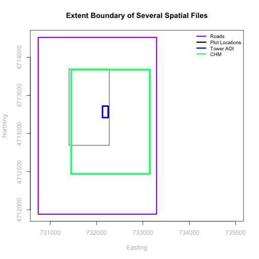
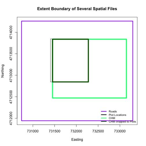
The graphic below illustrates the extent of several of the spatial layers that we have worked with in this vector data tutorial series:
- Area of interest (AOI) -- blue
- Roads and trails -- purple
- Vegetation plot locations -- black
and a raster file, that we will introduce this tutorial:
- A canopy height model (CHM) in GeoTIFF format -- green
Frequent use cases of cropping a raster file include reducing file size and creating maps.
Sometimes we have a raster file that is much larger than our study area or area of interest. In this case, it is often most efficient to crop the raster to the extent of our study area to reduce file sizes as we process our data.
Cropping a raster can also be useful when creating visually appealing maps so that the raster layer matches the extent of the desired vector layers.
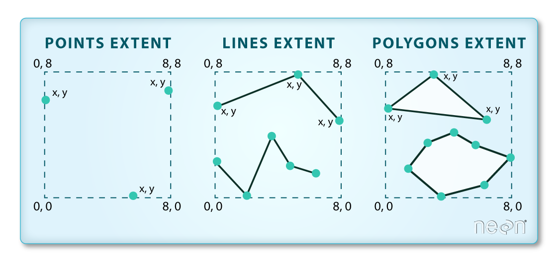
Import Data
We will begin by importing four vector shapefiles (field site boundary, roads/trails, tower location, and veg study plot locations) and one raster GeoTIFF file, a Canopy Height Model for the Harvard Forest, Massachusetts. These data can be used to create maps that characterize our study location.
If you have completed the Vector 00-04 tutorials in this Introduction to Working with Vector Data in R series, you can skip this code as you have already created these object.)
# load necessary packages
library(rgdal)  # for vector work; sp package should always load with rgdal.
library (raster)

# set working directory to data folder
# setwd("pathToDirHere")

# Imported in Vector 00: Vector Data in R - Open & Plot Data
# shapefile
aoiBoundary_HARV <- readOGR("NEON-DS-Site-Layout-Files/HARV/",
                            "HarClip_UTMZ18")
# Import a line shapefile
lines_HARV <- readOGR( "NEON-DS-Site-Layout-Files/HARV/",
                       "HARV_roads")
# Import a point shapefile
point_HARV <- readOGR("NEON-DS-Site-Layout-Files/HARV/",
                      "HARVtower_UTM18N")

# Imported in  Vector 02: .csv to Shapefile in R
# import raster Canopy Height Model (CHM)
chm_HARV <-
  raster("NEON-DS-Airborne-Remote-Sensing/HARV/CHM/HARV_chmCrop.tif")
Crop a Raster Using Vector Extent
We can use the crop function to crop a raster to the extent of another spatial
object. To do this, we need to specify the raster to be cropped and the spatial
object that will be used to crop the raster. R will use the extent of the
spatial object as the cropping boundary.
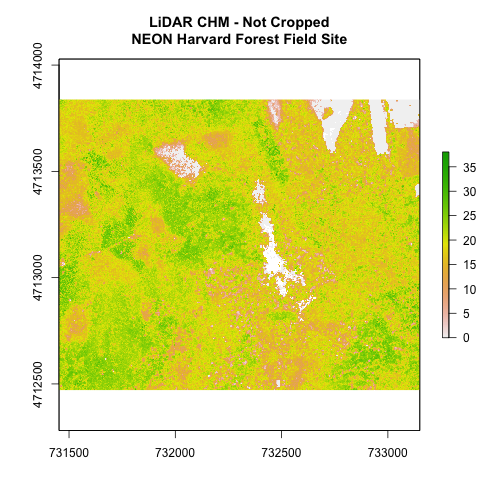
# plot full CHM
plot(chm_HARV,
     main="LiDAR CHM - Not Cropped\nNEON Harvard Forest Field Site")
# crop the chm
chm_HARV_Crop <- crop(x = chm_HARV, y = aoiBoundary_HARV)

# plot full CHM
plot(extent(chm_HARV),
     lwd=4,col="springgreen",
     main="LiDAR CHM - Cropped\nNEON Harvard Forest Field Site",
     xlab="easting", ylab="northing")

plot(chm_HARV_Crop,
     add=TRUE)
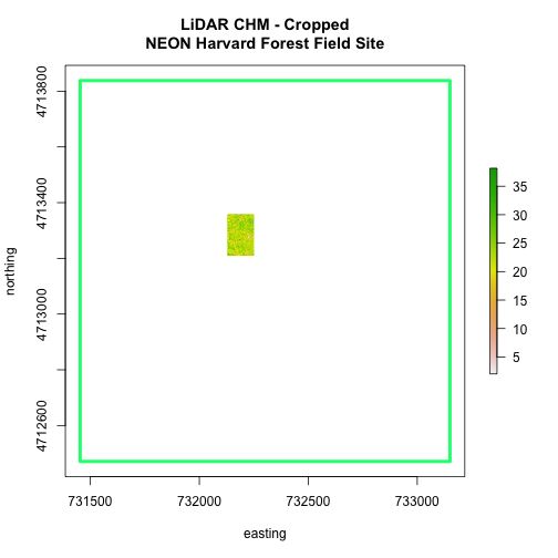
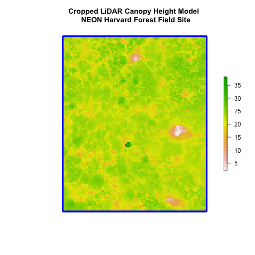
We can see from the plot above that the full CHM extent (plotted in green) is
much larger than the resulting cropped raster. Our new cropped CHM now has the
same extent as the aoiBoundary_HARV object that was used as a crop extent
(blue boarder below).
We can look at the extent of all the other objects.
# lets look at the extent of all of our objects
extent(chm_HARV)

## class      : Extent
## xmin       : 731453
## xmax       : 733150
## ymin       : 4712471
## ymax       : 4713838

extent(chm_HARV_Crop)

## class      : Extent
## xmin       : 732128
## xmax       : 732251
## ymin       : 4713209
## ymax       : 4713359

extent(aoiBoundary_HARV)

## class      : Extent
## xmin       : 732128
## xmax       : 732251.1
## ymin       : 4713209
## ymax       : 4713359
Which object has the largest extent? Our plot location extent is not the largest but it is larger than the AOI Boundary. It would be nice to see our vegetation plot locations with the Canopy Height Model information.
- Crop the Canopy Height Model to the extent of the study plot locations.
- Plot the vegetation plot location points on top of the Canopy Height Model.
If you completed the
.csv to Shapefile in R tutorial
you have these plot locations as the spatial R spatial object
plot.locationsSp_HARV. Otherwise, import the locations from the
\HARV\PlotLocations_HARV.shp shapefile in the downloaded data.
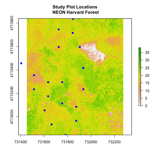
In the plot above, created in the challenge, all the vegetation plot locations (blue) appear on the Canopy Height Model raster layer except for one. One is situated on the white space. Why?
A modification of the first figure in this tutorial is below, showing the relative extents of all the spatial objects. Notice that the extent for our vegetation plot layer (black) extends further west than the extent of our CHM raster (bright green). The crop function will make a raster extent smaller, it will not expand the extent in areas where there are no data. Thus, extent of our vegetation plot layer will still extend further west than the extent of our (cropped) raster data (dark green).
Define an Extent
We can also use an extent() method to define an extent to be used as a cropping
boundary. This creates an object of class extent.
# extent format (xmin,xmax,ymin,ymax)
new.extent <- extent(732161.2, 732238.7, 4713249, 4713333)
class(new.extent)

## [1] "Extent"
## attr(,"package")
## [1] "raster"
Once we have defined the extent, we can use the crop function to crop our
raster.
# crop raster
CHM_HARV_manualCrop <- crop(x = chm_HARV, y = new.extent)

# plot extent boundary and newly cropped raster
plot(aoiBoundary_HARV,
     main = "Manually Cropped Raster\n NEON Harvard Forest Field Site")
plot(new.extent,
     col="brown",
     lwd=4,
     add = TRUE)
plot(CHM_HARV_manualCrop,
     add = TRUE)
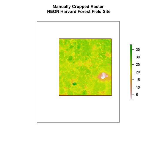
Notice that our manually set new.extent (in red) is smaller than the
aoiBoundary_HARV and that the raster is now the same as the new.extent
object.
See the documentation for the extent() function for more ways
to create an extent object using ??raster::extent
Extract Raster Pixels Values Using Vector Polygons
Often we want to extract values from a raster layer for particular locations - for example, plot locations that we are sampling on the ground.
To do this in R, we use the extract() function. The extract() function
requires:
- The raster that we wish to extract values from
- The vector layer containing the polygons that we wish to use as a boundary or boundaries
NOTE: We can tell it to store the output values in a data.frame using
df=TRUE (optional, default is to NOT return a data.frame) .
We will begin by extracting all canopy height pixel values located within our
aoiBoundary polygon which surrounds the tower located at the NEON Harvard
Forest field site.
# extract tree height for AOI
# set df=TRUE to return a data.frame rather than a list of values
tree_height <- raster::extract(x = chm_HARV,
                       y = aoiBoundary_HARV,
                       df = TRUE)

# view the object
head(tree_height)

##   ID HARV_chmCrop
## 1  1        21.20
## 2  1        23.85
## 3  1        23.83
## 4  1        22.36
## 5  1        23.95
## 6  1        23.89

nrow(tree_height)

## [1] 18450
When we use the extract command, R extracts the value for each pixel located
within the boundary of the polygon being used to perform the extraction, in
this case the aoiBoundary object (1 single polygon). Using the aoiBoundary as the boundary polygon, the
function extracted values from 18,450 pixels.
The extract function returns a list of values as default, but you can tell R
to summarize the data in some way or to return the data as a data.frame
(df=TRUE).
We can create a histogram of tree height values within the boundary to better
understand the structure or height distribution of trees. We can also use the
summary() function to view descriptive statistics including min, max and mean
height values to help us better understand vegetation at our field
site.
# view histogram of tree heights in study area
hist(tree_height$HARV_chmCrop,
     main="Histogram of CHM Height Values (m) \nNEON Harvard Forest Field Site",
     col="springgreen",
     xlab="Tree Height", ylab="Frequency of Pixels")
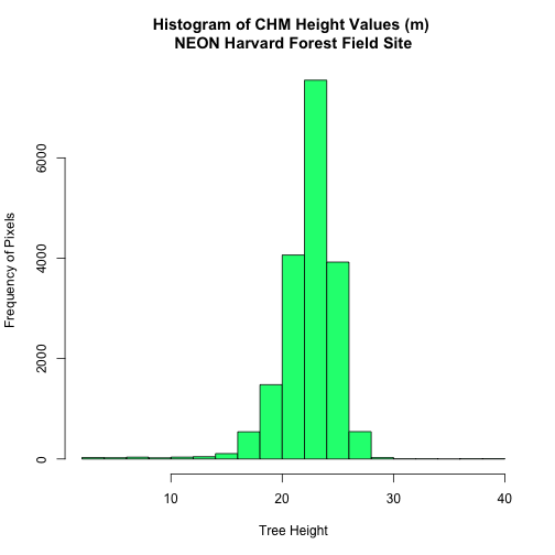
# view summary of values
summary(tree_height$HARV_chmCrop)

##    Min. 1st Qu.  Median    Mean 3rd Qu.    Max.
##    2.03   21.36   22.81   22.43   23.97   38.17
- Check out the documentation for the
extract()function for more details (??raster::extract).
Summarize Extracted Raster Values
We often want to extract summary values from a raster. We can tell R the type
of summary statistic we are interested in using the fun= method. Let's extract
a mean height value for our AOI.
# extract the average tree height (calculated using the raster pixels)
# located within the AOI polygon
av_tree_height_AOI <- raster::extract(x = chm_HARV,
                              y = aoiBoundary_HARV,
                              fun=mean,
                              df=TRUE)

# view output
av_tree_height_AOI

##   ID HARV_chmCrop
## 1  1     22.43018
It appears that the mean height value, extracted from our LiDAR data derived canopy height model is 22.43 meters.
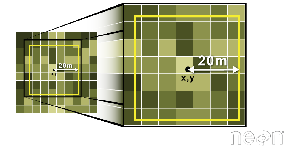
Extract Data using x,y Locations
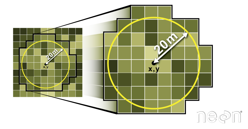
We can also extract pixel values from a raster by defining a buffer or area
surrounding individual point locations using the extract() function. To do this
we define the summary method (fun=mean) and the buffer distance (buffer=20)
which represents the radius of a circular region around each point.
The units of the buffer are the same units of the data CRS.
Let's put this into practice by figuring out the average tree height in the 20m around the tower location.
# what are the units of our buffer
crs(point_HARV)

## CRS arguments:
##  +proj=utm +zone=18 +datum=WGS84 +units=m +no_defs

# extract the average tree height (height is given by the raster pixel value)
# at the tower location
# use a buffer of 20 meters and mean function (fun)
av_tree_height_tower <- raster::extract(x = chm_HARV,
                                y = point_HARV,
                                buffer=20,
                                fun=mean,
                                df=TRUE)

# view data
head(av_tree_height_tower)

##   ID HARV_chmCrop
## 1  1     22.38812

# how many pixels were extracted
nrow(av_tree_height_tower)

## [1] 1
Use the plot location points shapefile HARV/plot.locations_HARV.shp or spatial
object plot.locationsSp_HARV to extract an average tree height value for the
area within 20m of each vegetation plot location in the study area.
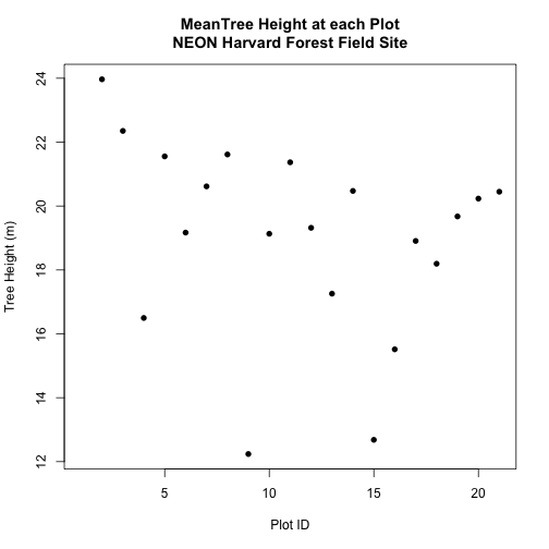
Create a simple plot showing the mean tree height of each plot using the plot()
function in base-R.