Intro to dplyr

When working with data frames in R, it is often useful to manipulate and summarize data. The dplyr package in R offers one of the most comprehensive group of functions to perform common manipulation tasks. In addition, the dplyr functions are often of a simpler syntax than most other data manipulation functions in R.

Elements of dplyr

There are several elements of dplyr that are unique to the library, and that do very cool things!

Functions for manipulating data

The text below was exerpted from the R CRAN dpylr vignettes.

Dplyr aims to provide a function for each basic verb of data manipulating, like:

• filter() (and slice())
  • filter rows based on values in specified columns
• arrange()
  • sort data by values in specified columns
• select() (and rename())
  • view and work with data from only specified columns
• distinct()
  • view and work with only unique values from specified columns
• mutate() (and transmute())
  • add new data to the data frame
• summarise()
  • calculate specified summary statistics on data
• sample_n() and sample_frac()
  • return a random sample of rows

Format of function calls

The single table verb functions share these features:

• The first argument is a data.frame (or a dplyr special class tbl_df, known as a 'tibble').
  • dplyr can work with data.frames as is, but if you're dealing with large data it's worthwhile to convert them to a tibble, to avoid printing a lot of data to the screen. You can do this with the function
    as_tibble().
  • Calling the class function on a tibble will return the vector c("tbl_df", "tbl", "data.frame").
• The subsequent arguments describe how to manipulate the data (e.g., based on which columns, using which summary statistics), and you can refer to columns directly (without using $).
• The result is always a new tibble.
• Function calls do not generate 'side-effects'; you always have to assign the results to an object

Grouped operations

Certain functions (e.g., group_by, summarise, and other 'aggregate functions') allow you to get information for groups of data, in one fell swoop. This is like performing database functions with knowing SQL or any other db specific code. Powerful stuff!

Piping

We often need to get a subset of data using one function, and then use another function to do something with that subset (and we may do this multiple times). This leads to nesting functions, which can get messy and hard to keep track of. Enter 'piping', dplyr's way of feeding the output of one function into another, and so on, without the hassleof parentheses and brackets.

Let's say we want to start with the data frame my_data, apply function1(), then function2(), and then function3(). This is what that looks like without piping:

function3(function2(function1(my_data)))

This is messy, difficult to read, and the reverse of the order our functions actually occur. If any of these functions needed additional arguments, the readability would be even worse!

The piping operator %>% takes everything in front of it and "pipes" it into the first argument of the function after. So now our example looks like this:

my_data %>%
  function1() %>%
  function2() %>%
  function3()

This runs identically to the original nested version!

For example, if we want to find the mean body weight of male mice, we'd do this:

	myMammalData %>%                     # start with a data frame
		filter(sex=='M') %>%               # first filter for rows where sex is male
		summarise (mean_weight = mean(weight))  # find the mean of the weight 
                                            # column, store as mean_weight

This is read as "from data frame myMammalData, select only males and return the mean weight as a new list mean_weight".

Download Small Mammal Data

Before we get started, we will need to download our data to investigate. To do so, we will use the loadByProduct() function from the neonUtilities package to download data straight from the NEON servers. To learn more about this function, please see the Download and Explore NEON data tutorial here.

Let's look at the NEON small mammal capture data from Harvard Forest (within Domain 01) for all of 2014. This site is located in the heart of the Lyme disease epidemic.

Read more about NEON terrestrial measurements here.

# load packages
library(dplyr)
library(neonUtilities)

# load the NEON small mammal capture data
# NOTE: the check.size = TRUE argument means the function 
# will require confirmation from you that you want to load 
# the quantity of data requested
loadData <- loadByProduct(dpID="DP1.10072.001", site = "HARV", 
                 startdate = "2014-01", enddate = "2014-12", 
                 check.size = TRUE) # Console requires your response!

# if you'd like, check out the data
str(loadData)

The loadByProduct() function calls the NEON server, downloads the monthly data files, and 'stacks' them together to form two tables of data called 'mam_pertrapnight' and 'mam_perplotnight'. It also saves the readme file, explanations of variables, and validation metadata, and combines these all into a single 'list' that we called 'loadData'. The only part of this list that we really need for this tutorial is the 'mam_pertrapnight' table, so let's extract just that one and call it 'myData'.

myData <- loadData$mam_pertrapnight

class(myData) # Confirm that 'myData' is a data.frame

## [1] "data.frame"

Use dplyr

For the rest of this tutorial, we are only going to be working with three variables within 'myData':

• scientificName a string of "Genus species"
• sex a string with "F", "M", or "U"
• identificationQualifier a string noting uncertainty in the species identification

filter()

This function:

• extracts only a subset of rows from a data frame according to specified conditions
• is similar to the base function subset(), but with simpler syntax
• inputs: data object, any number of conditional statements on the named columns of the data object
• output: a data object of the same class as the input object (e.g., data.frame in, data.frame out) with only those rows that meet the conditions

For example, let's create a new dataframe that contains only female Peromyscus mainculatus, one of the key small mammal players in the life cycle of Lyme disease-causing bacterium.

# filter on `scientificName` is Peromyscus maniculatus and `sex` is female. 
# two equals signs (==) signifies "is"
data_PeroManicFemales <- filter(myData, 
                   scientificName == 'Peromyscus maniculatus', 
                   sex == 'F')

# Note how we were able to put multiple conditions into the filter statement,
# pretty cool!

So we have a dataframe with our female P. mainculatus but how many are there?

# how many female P. maniculatus are in the dataset
# would could simply count the number of rows in the new dataset
nrow(data_PeroManicFemales)

## [1] 98

# or we could write is as a sentence
print(paste('In 2014, NEON technicians captured',
                   nrow(data_PeroManicFemales),
                   'female Peromyscus maniculatus at Harvard Forest.',
                   sep = ' '))

## [1] "In 2014, NEON technicians captured 98 female Peromyscus maniculatus at Harvard Forest."

That's awesome that we can quickly and easily count the number of female Peromyscus maniculatus that were captured at Harvard Forest in 2014. However, there is a slight problem. There are two Peromyscus species that are common in Harvard Forest: Peromyscus maniculatus (deer mouse) and Peromyscus leucopus (white-footed mouse). These species are difficult to distinguish in the field, leading to some uncertainty in the identification, which is noted in the 'identificationQualifier' data field by the term "cf. species" or "aff. species". (For more information on these terms and 'open nomenclature' please see this great Wiki article here). When the field technician is certain of their identification (or if they forget to note their uncertainty), identificationQualifier will be NA. Let's run the same code as above, but this time specifying that we want only those observations that are unambiguous identifications.

# filter on `scientificName` is Peromyscus maniculatus and `sex` is female. 
# two equals signs (==) signifies "is"
data_PeroManicFemalesCertain <- filter(myData, 
                   scientificName == 'Peromyscus maniculatus', 
                   sex == 'F',
                   identificationQualifier =="NA")

# Count the number of un-ambiguous identifications
nrow(data_PeroManicFemalesCertain)

## [1] 0

Woah! So every single observation of a Peromyscus maniculatus had some level of uncertainty that the individual may actually be Peromyscus leucopus. This is understandable given the difficulty of field identification for these species. Given this challenge, it will be best for us to consider these mice at the genus level. We can accomplish this by searching for only the genus name in the 'scientificName' field using the grepl() function.

grepl()

This is a function in the base package (e.g., it isn't part of dplyr) that is part of the suite of Regular Expressions functions. grepl uses regular expressions to match patterns in character strings. Regular expressions offer very powerful and useful tricks for data manipulation. They can be complicated and therefore are a challenge to learn, but well worth it!

Here, we present a very simple example.

• inputs: pattern to match, character vector to search for a match
• output: a logical vector indicating whether the pattern was found within each element of the input character vector

Let's use grepl to learn more about our possible disease vectors. In reality, all species of Peromyscus are viable players in Lyme disease transmission, and they are difficult to distinguise in a field setting, so we really should be looking at all species of Peromyscus. Since we don't have genera split out as a separate field, we have to search within the scientificName string for the genus -- this is a simple example of pattern matching.

We can use the dplyr function filter() in combination with the base function grepl() to accomplish this.

# combine filter & grepl to get all Peromyscus (a part of the 
# scientificName string)
data_PeroFemales <- filter(myData,
                   grepl('Peromyscus', scientificName),
                   sex == 'F')

# how many female Peromyscus are in the dataset
print(paste('In 2014, NEON technicians captured',
                   nrow(data_PeroFemales),
                   'female Peromyscus spp. at Harvard Forest.',
                   sep = ' '))

## [1] "In 2014, NEON technicians captured 558 female Peromyscus spp. at Harvard Forest."

group_by() + summarise()

An alternative to using the filter function to subset the data (and make a new data object in the process), is to calculate summary statistics based on some grouping factor. We'll use group_by(), which does basically the same thing as SQL or other tools for interacting with relational databases. For those unfamiliar with SQL, no worries - dplyr provides lots of additional functionality for working with databases (local and remote) that does not require knowledge of SQL. How handy!

The group_by() function in dplyr allows you to perform functions on a subset of a dataset without having to create multiple new objects or construct for() loops. The combination of group_by() and summarise() are great for generating simple summaries (counts, sums) of grouped data.

NOTE: Be continentious about using summarise with other summary functions! You need to think about weighting for means and variances, and summarize doesn't work precisely for medians if there is any missing data (e.g., if there was no value recorded, maybe it was for a good reason!).

Continuing with our small mammal data, since the diversity of the entire small mammal community has been shown to impact disease dynamics among the key reservoir species, we really want to know more about the demographics of the whole community. We can quickly generate counts by species and sex in 2 lines of code, using group_by and summarise.

# how many of each species & sex were there?
# step 1: group by species & sex
dataBySpSex <- group_by(myData, scientificName, sex)

# step 2: summarize the number of individuals of each using the new df
countsBySpSex <- summarise(dataBySpSex, n_individuals = n())

## `summarise()` regrouping output by 'scientificName' (override with `.groups` argument)

# view the data (just top 10 rows)
head(countsBySpSex, 10)

## # A tibble: 10 x 3
## # Groups:   scientificName [5]
##    scientificName          sex   n_individuals
##    <chr>                   <chr>         <int>
##  1 Blarina brevicauda      F                50
##  2 Blarina brevicauda      M                 8
##  3 Blarina brevicauda      U                22
##  4 Blarina brevicauda      <NA>             19
##  5 Glaucomys volans        M                 1
##  6 Mammalia sp.            U                 1
##  7 Mammalia sp.            <NA>              1
##  8 Microtus pennsylvanicus F                 2
##  9 Myodes gapperi          F               103
## 10 Myodes gapperi          M                99

Note: the output of step 1 (dataBySpSex) does not look any different than the original dataframe (myData), but the application of subsequent functions (e.g., summarise) to this new dataframe will produce distinctly different results than if you tried the same operations on the original. Try it if you want to see the difference! This is because the group_by() function converted dataBySpSex into a "grouped_df" rather than just a "data.frame". In order to confirm this, try using the class() function on both myData and dataBySpSex. You can also read the help documentation for this function by running the code: ?group_by()

# View class of 'myData' object
class(myData)

## [1] "data.frame"

# View class of 'dataBySpSex' object
class(dataBySpSex)

## [1] "grouped_df" "tbl_df"     "tbl"        "data.frame"

# View help file for group_by() function
?group_by()

Pipe functions together

We created multiple new data objects during our explorations of dplyr functions, above. While this works, we can produce the same results more efficiently by chaining functions together and creating only one new data object that encapsulates all of the previously sought information: filter on only females, grepl to get only Peromyscus spp., group_by individual species, and summarise the numbers of individuals.

# combine several functions to get a summary of the numbers of individuals of 
# female Peromyscus species in our dataset.

# remember %>% are "pipes" that allow us to pass information from one function 
# to the next. 

dataBySpFem <- myData %>% 
                  filter(grepl('Peromyscus', scientificName), sex == "F") %>%
                  group_by(scientificName) %>%
                  summarise(n_individuals = n())

## `summarise()` ungrouping output (override with `.groups` argument)

# view the data
dataBySpFem

## # A tibble: 3 x 2
##   scientificName         n_individuals
##   <chr>                          <int>
## 1 Peromyscus leucopus              455
## 2 Peromyscus maniculatus            98
## 3 Peromyscus sp.                     5

Cool!

Base R only

So that is nice, but we had to install a new package dplyr. You might ask, "Is it really worth it to learn new commands if I can do this is base R." While we think "yes", why don't you see for yourself. Here is the base R code needed to accomplish the same task.

# For reference, the same output but using R's base functions

# First, subset the data to only female Peromyscus
dataFemPero  <- myData[myData$sex == 'F' & 
                   grepl('Peromyscus', myData$scientificName), ]

# Option 1 --------------------------------
# Use aggregate and then rename columns
dataBySpFem_agg <-aggregate(dataFemPero$sex ~ dataFemPero$scientificName, 
                   data = dataFemPero, FUN = length)
names(dataBySpFem_agg) <- c('scientificName', 'n_individuals')

# view output
dataBySpFem_agg

##           scientificName n_individuals
## 1    Peromyscus leucopus           455
## 2 Peromyscus maniculatus            98
## 3         Peromyscus sp.             5

# Option 2 --------------------------------------------------------
# Do it by hand

# Get the unique scientificNames in the subset
sppInDF <- unique(dataFemPero$scientificName[!is.na(dataFemPero$scientificName)])

# Use a loop to calculate the numbers of individuals of each species
sciName <- vector(); numInd <- vector()
for (i in sppInDF) {
  sciName <- c(sciName, i)
  numInd <- c(numInd, length(which(dataFemPero$scientificName==i)))
}

#Create the desired output data frame
dataBySpFem_byHand <- data.frame('scientificName'=sciName, 
                   'n_individuals'=numInd)

# view output
dataBySpFem_byHand

##           scientificName n_individuals
## 1    Peromyscus leucopus           455
## 2 Peromyscus maniculatus            98
## 3         Peromyscus sp.             5

About Hierarchical Data Formats - HDF5

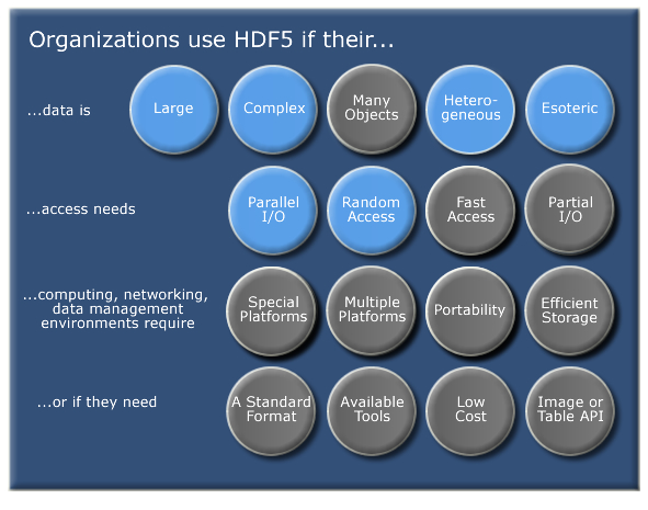
The Hierarchical Data Format version 5 (HDF5), is an open source file format that supports large, complex, heterogeneous data. HDF5 uses a "file directory" like structure that allows you to organize data within the file in many different structured ways, as you might do with files on your computer. The HDF5 format also allows for embedding of metadata making it self-describing.

Hierarchical Structure - A file directory within a file

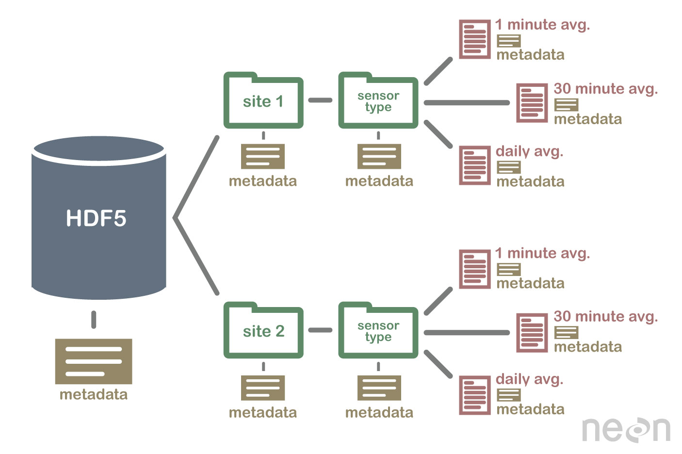
The HDF5 format can be thought of as a file system contained and described within one single file. Think about the files and folders stored on your computer. You might have a data directory with some temperature data for multiple field sites. These temperature data are collected every minute and summarized on an hourly, daily and weekly basis. Within one HDF5 file, you can store a similar set of data organized in the same way that you might organize files and folders on your computer. However in a HDF5 file, what we call "directories" or "folders" on our computers, are called groups and what we call files on our computer are called datasets.

2 Important HDF5 Terms

• Group: A folder like element within an HDF5 file that might contain other groups OR datasets within it.
• Dataset: The actual data contained within the HDF5 file. Datasets are often (but don't have to be) stored within groups in the file.

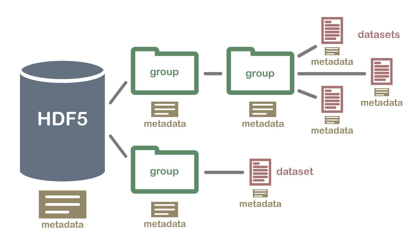
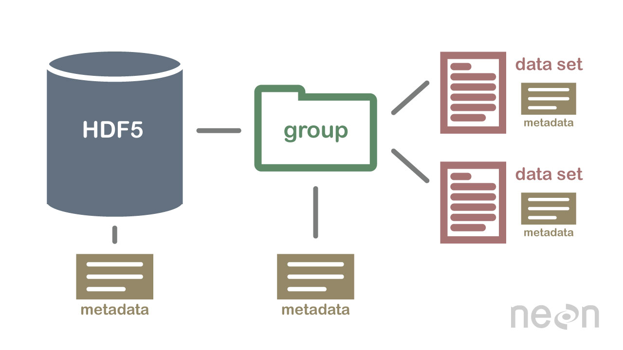
An HDF5 file containing datasets, might be structured like this:

HDF5 is a Self Describing Format

HDF5 format is self describing. This means that each file, group and dataset can have associated metadata that describes exactly what the data are. Following the example above, we can embed information about each site to the file, such as:

• The full name and X,Y location of the site
• Description of the site.
• Any documentation of interest.

Similarly, we might add information about how the data in the dataset were collected, such as descriptions of the sensor used to collect the temperature data. We can also attach information, to each dataset within the site group, about how the averaging was performed and over what time period data are available.

One key benefit of having metadata that are attached to each file, group and dataset, is that this facilitates automation without the need for a separate (and additional) metadata document. Using a programming language, like R or Python, we can grab information from the metadata that are already associated with the dataset, and which we might need to process the dataset.

Compressed & Efficient subsetting

The HDF5 format is a compressed format. The size of all data contained within HDF5 is optimized which makes the overall file size smaller. Even when compressed, however, HDF5 files often contain big data and can thus still be quite large. A powerful attribute of HDF5 is data slicing, by which a particular subsets of a dataset can be extracted for processing. This means that the entire dataset doesn't have to be read into memory (RAM); very helpful in allowing us to more efficiently work with very large (gigabytes or more) datasets!

Heterogeneous Data Storage

HDF5 files can store many different types of data within in the same file. For example, one group may contain a set of datasets to contain integer (numeric) and text (string) data. Or, one dataset can contain heterogeneous data types (e.g., both text and numeric data in one dataset). This means that HDF5 can store any of the following (and more) in one file:

• Temperature, precipitation and PAR (photosynthetic active radiation) data for a site or for many sites
• A set of images that cover one or more areas (each image can have specific spatial information associated with it - all in the same file)
• A multi or hyperspectral spatial dataset that contains hundreds of bands.
• Field data for several sites characterizing insects, mammals, vegetation and climate.
• A set of images that cover one or more areas (each image can have unique spatial information associated with it)
• And much more!

Open Format

The HDF5 format is open and free to use. The supporting libraries (and a free viewer), can be downloaded from the HDF Group website. As such, HDF5 is widely supported in a host of programs, including open source programming languages like R and Python, and commercial programming tools like Matlab and IDL. Spatial data that are stored in HDF5 format can be used in GIS and imaging programs including QGIS, ArcGIS, and ENVI.

Summary Points - Benefits of HDF5

• Self-Describing The datasets with an HDF5 file are self describing. This allows us to efficiently extract metadata without needing an additional metadata document.
• Supporta Heterogeneous Data: Different types of datasets can be contained within one HDF5 file.
• Supports Large, Complex Data: HDF5 is a compressed format that is designed to support large, heterogeneous, and complex datasets.
• Supports Data Slicing: "Data slicing", or extracting portions of the dataset as needed for analysis, means large files don't need to be completely read into the computers memory or RAM.
• Open Format - wide support in the many tools: Because the HDF5 format is open, it is supported by a host of programming languages and tools, including open source languages like R and Python and open GIS tools like QGIS.

In this tutorial you will use the free HDFView tool to explore HDF5 files and the groups and datasets contained within. You will also see how HDF5 files can be structured and explore metadata using both spatial and temporal data stored in HDF5!

Installing HDFView

Select the HDFView download option that matches the operating system (Mac OS X, Windows, or Linux) and computer setup (32 bit vs 64 bit) that you have.

This tutorial was written with graphics from the VS 2012 version, but it is applicable to other versions as well.

Hierarchical Data Format 5 - HDF5

Hierarchical Data Format version 5 (HDF5), is an open file format that supports large, complex, heterogeneous data. Some key points about HDF5:

• HDF5 uses a "file directory" like structure.
• The HDF5 data models organizes information using Groups. Each group may contain one or more datasets.
• HDF5 is a self describing file format. This means that the metadata for the data contained within the HDF5 file, are built into the file itself.
• One HDF5 file may contain several heterogeneous data types (e.g. images, numeric data, data stored as strings).

For more introduction to the HDF5 format, see our About Hierarchical Data Formats - What is HDF5? tutorial.

In this tutorial, we will explore two different types of data saved in HDF5. This will allow us to better understand how one file can store multiple different types of data, in different ways.

Part 1: Exploring Temperature Data in HDF5 Format in HDFView

The first thing that we will do is open an HDF5 file in the viewer to get a better idea of how HDF5 files can be structured.

Open a HDF5/H5 file in HDFView

To begin, open the HDFView application. Within the HDFView application, select File --> Open and navigate to the folder where you saved the NEONDSTowerTemperatureData.hdf5 file on your computer. Open this file in HDFView.

If you click on the name of the HDF5 file in the left hand window of HDFView, you can view metadata for the file. This will be located in the bottom window of the application.

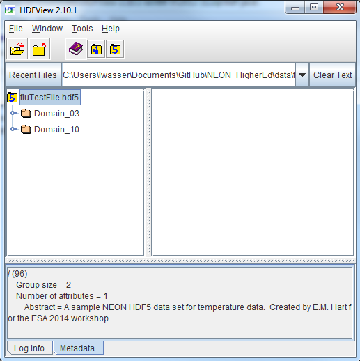
Explore File Structure in HDFView

Next, explore the structure of this file. Notice that there are two Groups (represented as folder icons in the viewer) called "Domain_03" and "Domain_10". Within each domain group, there are site groups (NEON sites that are located within those domains). Expand these folders by double clicking on the folder icons. Double clicking expands the groups content just as you might expand a folder in Windows explorer.

Notice that there is metadata associated with each group.

Double click on the OSBS group located within the Domain_03 group. Notice in the metadata window that OSBS contains data collected from the NEON Ordway-Swisher Biological Station field site.

Within the OSBS group there are two more groups - Min_1 and Min_30. What data are contained within these groups?

Expand the "min_1" group within the OSBS site in Domain_03. Notice that there are five more nested groups named "Boom_1, 2, etc". A boom refers to an arm on a tower, which sits at a particular height and to which are attached sensors for collecting data on such variables as temperature, wind speed, precipitation, etc. In this case, we are working with data collected using temperature sensors, mounted on the tower booms.

Speaking of temperature - what type of sensor is collected the data within the boom_1 folder at the Ordway Swisher site? HINT: check the metadata for that dataset.

Expand the "Boom_1" folder by double clicking it. Finally, we have arrived at a dataset! Have a look at the metadata associated with the temperature dataset within the boom_1 group. Notice that there is metadata describing each attribute in the temperature dataset. Double click on the group name to open up the table in a tabular format. Notice that these data are temporal.

So this is one example of how an HDF5 file could be structured. This particular file contains data from multiple sites, collected from different sensors (mounted on different booms on the tower) and collected over time. Take some time to explore this HDF5 dataset within the HDFViewer.

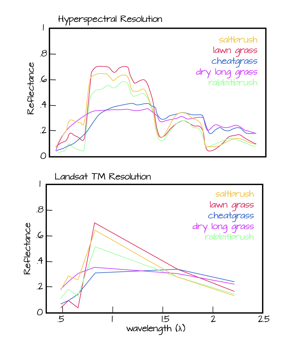
Part 2: Exploring Hyperspectral Imagery stored in HDF5

Next, we will explore a hyperspectral dataset, collected by the NEON Airborne Observation Platform (AOP) and saved in HDF5 format. Hyperspectral data are naturally hierarchical, as each pixel in the dataset contains reflectance values for hundreds of bands collected by the sensor. The NEON sensor (imaging spectrometer) collected data within 428 bands.

A few notes about hyperspectral imagery:

• An imaging spectrometer, which collects hyperspectral imagery, records light energy reflected off objects on the earth's surface.
• The data are inherently spatial. Each "pixel" in the image is located spatially and represents an area of ground on the earth.
• Similar to an Red, Green, Blue (RGB) camera, an imaging spectrometer records reflected light energy. Each pixel will contain several hundred bands worth of reflectance data.

Read more about hyperspectral remote sensing data:

• About Hyperspectral Remote Sensing Data tutorial on this site.
• White paper by Dr Peg Shippert

Let's open some hyperspectral imagery stored in HDF5 format to see what the file structure can like for a different type of data.

Open the file. Notice that it is structured differently. This file is composed of 3 datasets:

• Reflectance,
• fwhm, and
• wavelength.

It also contains some text information called "map info". Finally it contains a group called spatial info.

Let's first look at the metadata stored in the spatialinfo group. This group contains all of the spatial information that a GIS program would need to project the data spatially.

Next, double click on the wavelength dataset. Note that this dataset contains the central wavelength value for each band in the dataset.

Finally, click on the reflectance dataset. Note that in the metadata for the dataset that the structure of the dataset is 426 x 501 x 477 (wavelength, line, sample), as indicated in the metadata. Right click on the reflectance dataset and select Open As. Click Image in the "display as" settings on the left hand side of the popup.

In this case, the image data are in the second and third dimensions of this dataset. However, HDFView will default to selecting the first and second dimensions

Let’s tell the HDFViewer to use the second and third dimensions to view the image:

1. Under height, make sure dim 1 is selected.
2. Under width, make sure dim 2 is selected.

Notice an image preview appears on the left of the pop-up window. Click OK to open the image. You may have to play with the brightness and contrast settings in the viewer to see the data properly.

Explore the spectral dataset in the HDFViewer taking note of the metadata and data stored within the file.

About HDF5

The HDF5 file can store large, heterogeneous datasets that include metadata. It also supports efficient data slicing, or extraction of particular subsets of a dataset which means that you don't have to read large files read into the computers memory / RAM in their entirety in order work with them.

Read more about HDF5 here.

HDF5 in R

To access HDF5 files in R, we will use the rhdf5 library which is part of the Bioconductor suite of R libraries. It might also be useful to install the free HDF5 viewer which will allow you to explore the contents of an HDF5 file using a graphic interface.

More about working with HDFview and a hands-on activity here.

First, let's get R setup. We will use the rhdf5 library. To access HDF5 files in R, we will use the rhdf5 library which is part of the Bioconductor suite of R packages. As of May 2020 this package was not yet on CRAN.

# Install rhdf5 package (only need to run if not already installed)
#install.packages("BiocManager")
#BiocManager::install("rhdf5")

# Call the R HDF5 Library
library("rhdf5")

# set working directory to ensure R can find the file we wish to import and where
# we want to save our files
wd <- "~/Git/data/" #This will depend on your local environment 
setwd(wd) 

Read more about the rhdf5 package here.

Create an HDF5 File in R

Now, let's create a basic H5 file with one group and one dataset in it.

# Create hdf5 file
h5createFile("vegData.h5")

## [1] TRUE

# create a group called aNEONSite within the H5 file
h5createGroup("vegData.h5", "aNEONSite")

## [1] TRUE

# view the structure of the h5 we've created
h5ls("vegData.h5")

##   group      name     otype dclass dim
## 0     / aNEONSite H5I_GROUP

Next, let's create some dummy data to add to our H5 file.

# create some sample, numeric data 
a <- rnorm(n=40, m=1, sd=1) 
someData <- matrix(a,nrow=20,ncol=2)

Write the sample data to the H5 file.

# add some sample data to the H5 file located in the aNEONSite group
# we'll call the dataset "temperature"
h5write(someData, file = "vegData.h5", name="aNEONSite/temperature")

# let's check out the H5 structure again
h5ls("vegData.h5")

##        group        name       otype dclass    dim
## 0          /   aNEONSite   H5I_GROUP              
## 1 /aNEONSite temperature H5I_DATASET  FLOAT 20 x 2

View a "dump" of the entire HDF5 file. NOTE: use this command with CAUTION if you are working with larger datasets!

# we can look at everything too 
# but be cautious using this command!
h5dump("vegData.h5")

## $aNEONSite
## $aNEONSite$temperature
##              [,1]       [,2]
##  [1,]  0.33155432  2.4054446
##  [2,]  1.14305151  1.3329978
##  [3,] -0.57253964  0.5915846
##  [4,]  2.82950139  0.4669748
##  [5,]  0.47549005  1.5871517
##  [6,] -0.04144519  1.9470377
##  [7,]  0.63300177  1.9532294
##  [8,] -0.08666231  0.6942748
##  [9,] -0.90739256  3.7809783
## [10,]  1.84223101  1.3364965
## [11,]  2.04727590  1.8736805
## [12,]  0.33825921  3.4941913
## [13,]  1.80738042  0.5766373
## [14,]  1.26130759  2.2307994
## [15,]  0.52882731  1.6021497
## [16,]  1.59861449  0.8514808
## [17,]  1.42037674  1.0989390
## [18,] -0.65366487  2.5783750
## [19,]  1.74865593  1.6069304
## [20,] -0.38986048 -1.9471878

# Close the file. This is good practice.
H5close()

Add Metadata (attributes)

Let's add some metadata (called attributes in HDF5 land) to our dummy temperature data. First, open up the file.

# open the file, create a class
fid <- H5Fopen("vegData.h5")
# open up the dataset to add attributes to, as a class
did <- H5Dopen(fid, "aNEONSite/temperature")

# Provide the NAME and the ATTR (what the attribute says) for the attribute.
h5writeAttribute(did, attr="Here is a description of the data",
                 name="Description")
h5writeAttribute(did, attr="Meters",
                 name="Units")

Now we can add some attributes to the file.

# let's add some attributes to the group
did2 <- H5Gopen(fid, "aNEONSite/")

h5writeAttribute(did2, attr="San Joaquin Experimental Range",
                 name="SiteName")

h5writeAttribute(did2, attr="Southern California",
                 name="Location")

# close the files, groups and the dataset when you're done writing to them!
H5Dclose(did)

H5Gclose(did2)

H5Fclose(fid)

Working with an HDF5 File in R

Now that we've created our H5 file, let's use it! First, let's have a look at the attributes of the dataset and group in the file.

# look at the attributes of the precip_data dataset
h5readAttributes(file = "vegData.h5", 
                 name = "aNEONSite/temperature")

## $Description
## [1] "Here is a description of the data"
## 
## $Units
## [1] "Meters"

# look at the attributes of the aNEONsite group
h5readAttributes(file = "vegData.h5", 
                 name = "aNEONSite")

## $Location
## [1] "Southern California"
## 
## $SiteName
## [1] "San Joaquin Experimental Range"

# let's grab some data from the H5 file
testSubset <- h5read(file = "vegData.h5", 
                 name = "aNEONSite/temperature")

testSubset2 <- h5read(file = "vegData.h5", 
                 name = "aNEONSite/temperature",
                 index=list(NULL,1))
H5close()

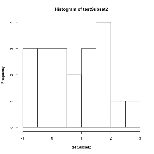
Once we've extracted data from our H5 file, we can work with it in R.

# create a quick plot of the data
hist(testSubset2)