This is a tutorial in pulling data from the NEON API or Application Programming Interface. The tutorial uses R and the R package httr, but the core information about the API is applicable to other languages and approaches.

What is an API?

If you are unfamiliar with the concept of an API, think of an API as a ‘middle person' that provides a communication path for a software application to obtain information from a digital data source. APIs are becoming a very common means of sharing digital information. Many of the apps that you use on your computer or mobile device to produce maps, charts, reports, and other useful forms of information pull data from multiple sources using APIs. In the ecological and environmental sciences, many researchers use APIs to programmatically pull data into their analyses. (Quoted from the NEON Observatory Blog story: API and data availability viewer now live on the NEON data portal.)

What is accessible via the NEON API?

The NEON API includes endpoints for NEON data and metadata, including spatial data, taxonomic data, and samples (see Endpoints below). This tutorial explores these sources of information using a specific data product as a guide. The principles and rule sets described below can be applied to other data products and metadata.

Anatomy of an API call

An example API call: http://data.neonscience.org/api/v0/data/DP1.10003.001/WOOD/2015-07

This includes the base URL, endpoint, and target.

Base URL:

http://data.neonscience.org/api/v0/data/DP1.10003.001/WOOD/2015-07

Specifics are appended to this in order to get the data or metadata you're looking for, but all calls to an API will include the base URL. For the NEON API, this is http://data.neonscience.org/api/v0 -- not clickable, because the base URL by itself will take you nowhere!

Endpoints:

http://data.neonscience.org/api/v0/data/DP1.10098.001/WOOD/2015-07

What type of data or metadata are you looking for?

• ~/products Information about one or all of NEON's data products

• ~/sites Information about data availability at the site specified in the call

• ~/locations Spatial data for the NEON locations specified in the call

• ~/data Data! By product, site, and date (in monthly chunks)

• ~/samples Information about sample relationships and sample tracking

• ~/taxonomy Access to NEON's taxon lists, the approved scientific names for sampled taxa

Targets:

http://data.neonscience.org/api/v0/data/DP1.10098.001/WOOD/2015-07

The specific data product, location, sample, etc, you want to get data for.

Data, by way of Products

Which product do you want to get data for? Consult the Explore Data Products page.

We'll pick Woody vegetation structure, DP1.10098.001

Your first thought is probably to use the /data endpoint. And we'll get there. But notice above that the API call for the /data endpoint includes the site and month of data to download. You don't want to have to guess sites and months at random - first, you need to see which sites and months have available data for the product you're interested in. That can be done either through the /sites or the /products endpoint; here we'll use /products.

Note: Checking for data availability can sometimes be skipped for the streaming sensor data products. In general, they are available continuously, and you could theoretically query a site and month of interest and expect there to be data by default. However, there can be interruptions to sensor data, in particular at aquatic sites, so checking availability first is the most reliable approach.

Use the products endpoint to query for Woody vegetation data. The target is the data product identifier, noted above, DP1.10098.001:

# Load the necessary libraries
library(httr)
library(jsonlite)

# Request data using the GET function & the API call
req <- GET("http://data.neonscience.org/api/v0/products/DP1.10098.001")
req

## Response [https://data.neonscience.org/api/v0/products/DP1.10098.001]
##   Date: 2021-06-16 01:03
##   Status: 200
##   Content-Type: application/json;charset=UTF-8
##   Size: 70.1 kB

The object returned from GET() has many layers of information. Entering the name of the object gives you some basic information about what you accessed. Status: 200 indicates this was a successful query; the status field can be a useful place to look if something goes wrong. These are HTTP status codes, you can google them to find out what a given value indicates.

The Content-Type parameter tells us we've accessed a json file. The easiest way to translate this to something more manageable in R is to use the fromJSON() function in the jsonlite package. It will convert the json into a nested list, flattening the nesting where possible.

# Make the data readable by jsonlite
req.text <- content(req, as="text")

# Flatten json into a nested list
avail <- jsonlite::fromJSON(req.text, 
                            simplifyDataFrame=T, 
                            flatten=T)

A lot of the content here is basic information about the data product. You can see all of it by running the line print(avail), but this will result in a very long printout in your console. Instead, try viewing list items individually. Here, we highlight a couple of interesting examples:

# View description of data product
avail$data$productDescription

## [1] "Structure measurements, including height, crown diameter, and stem diameter, as well as mapped position of individual woody plants"

# View data product abstract
avail$data$productAbstract

## [1] "This data product contains the quality-controlled, native sampling resolution data from in-situ measurements of live and standing dead woody individuals and shrub groups, from all terrestrial NEON sites with qualifying woody vegetation. The exact measurements collected per individual depend on growth form, and these measurements are focused on enabling biomass and productivity estimation, estimation of shrub volume and biomass, and calibration / validation of multiple NEON airborne remote-sensing data products. In general, comparatively large individuals that are visible to remote-sensing instruments are mapped, tagged and measured, and other smaller individuals are tagged and measured but not mapped. Smaller individuals may be subsampled according to a nested subplot approach in order to standardize the per plot sampling effort. Structure and mapping data are reported per individual per plot; sampling metadata, such as per growth form sampling area, are reported per plot. For additional details, see the user guide, protocols, and science design listed in the Documentation section in this data product's details webpage.\n\nLatency:\nThe expected time from data and/or sample collection in the field to data publication is as follows, for each of the data tables (in days) in the downloaded data package. See the Data Product User Guide for more information.\n\nvst_apparentindividual:  90\n\nvst_mappingandtagging:  90\n\nvst_perplotperyear:  300\n\nvst_shrubgroup:  90"

You may notice that some of this information is also accessible on the NEON data portal. The portal uses the same data sources as the API, and in many cases the portal is using the API on the back end, and simply adding a more user-friendly display to the data.

We want to find which sites and months have available data. That is in the siteCodes section. Let's look at what information is presented for each site:

# Look at the first list element for siteCode
avail$data$siteCodes$siteCode[[1]]

## [1] "ABBY"

# And at the first list element for availableMonths
avail$data$siteCodes$availableMonths[[1]]

##  [1] "2015-07" "2015-08" "2016-08" "2016-09" "2016-10" "2016-11" "2017-03" "2017-04" "2017-07" "2017-08"
## [11] "2017-09" "2018-07" "2018-08" "2018-09" "2018-10" "2018-11" "2019-07" "2019-09" "2019-10" "2019-11"

Here we can see the list of months with data for the site ABBY, which is the Abby Road forest in Washington state.

The section $data$siteCodes$availableDataUrls provides the exact API calls we need in order to query the data for each available site and month.

# Get complete list of available data URLs
wood.urls <- unlist(avail$data$siteCodes$availableDataUrls)

# Total number of URLs
length(wood.urls)

## [1] 535

# Show first 10 URLs available
wood.urls[1:10] 

##  [1] "https://data.neonscience.org/api/v0/data/DP1.10098.001/ABBY/2015-07"
##  [2] "https://data.neonscience.org/api/v0/data/DP1.10098.001/ABBY/2015-08"
##  [3] "https://data.neonscience.org/api/v0/data/DP1.10098.001/ABBY/2016-08"
##  [4] "https://data.neonscience.org/api/v0/data/DP1.10098.001/ABBY/2016-09"
##  [5] "https://data.neonscience.org/api/v0/data/DP1.10098.001/ABBY/2016-10"
##  [6] "https://data.neonscience.org/api/v0/data/DP1.10098.001/ABBY/2016-11"
##  [7] "https://data.neonscience.org/api/v0/data/DP1.10098.001/ABBY/2017-03"
##  [8] "https://data.neonscience.org/api/v0/data/DP1.10098.001/ABBY/2017-04"
##  [9] "https://data.neonscience.org/api/v0/data/DP1.10098.001/ABBY/2017-07"
## [10] "https://data.neonscience.org/api/v0/data/DP1.10098.001/ABBY/2017-08"

These URLs are the API calls we can use to find out what files are available for each month where there are data. They are pre-constructed calls to the /data endpoint of the NEON API.

Let's look at the woody plant data from the Rocky Mountain National Park (RMNP) site from October 2019. We can do this by using the GET() function on the relevant URL, which we can extract using the grep() function.

Note that if you want data from more than one site/month you need to iterate this code, GET() fails if you give it more than one URL at a time.

# Get available data for RMNP Oct 2019
woody <- GET(wood.urls[grep("RMNP/2019-10", wood.urls)])
woody.files <- jsonlite::fromJSON(content(woody, as="text"))

# See what files are available for this site and month
woody.files$data$files$name

## [1] "NEON.D10.RMNP.DP1.10098.001.EML.20191010-20191017.20210123T023002Z.xml"               
## [2] "NEON.D10.RMNP.DP1.10098.001.2019-10.basic.20210114T173951Z.zip"                       
## [3] "NEON.D10.RMNP.DP1.10098.001.vst_apparentindividual.2019-10.basic.20210114T173951Z.csv"
## [4] "NEON.D10.RMNP.DP1.10098.001.variables.20210114T173951Z.csv"                           
## [5] "NEON.D10.RMNP.DP0.10098.001.categoricalCodes.20210114T173951Z.csv"                    
## [6] "NEON.D10.RMNP.DP1.10098.001.readme.20210123T023002Z.txt"                              
## [7] "NEON.D10.RMNP.DP1.10098.001.vst_perplotperyear.2019-10.basic.20210114T173951Z.csv"    
## [8] "NEON.D10.RMNP.DP1.10098.001.vst_mappingandtagging.basic.20210114T173951Z.csv"         
## [9] "NEON.D10.RMNP.DP0.10098.001.validation.20210114T173951Z.csv"

If you've downloaded NEON data before via the data portal or the neonUtilities package, this should look very familiar. The format for most of the file names is:

NEON.[domain number].[site code].[data product ID].[file-specific name]. [year and month of data].[basic or expanded data package]. [date of file creation]

Some files omit the year and month, and/or the data package, since they're not specific to a particular measurement interval, such as the data product readme and variables files. The date of file creation uses the ISO6801 format, for example 20210114T173951Z, and can be used to determine whether data have been updated since the last time you downloaded.

Available files in our query for October 2019 at Rocky Mountain are all of the following (leaving off the initial NEON.D10.RMNP.DP1.10098.001):

• ~.vst_perplotperyear.2019-10.basic.20210114T173951Z.csv: data table of measurements conducted at the plot level every year

• ~.vst_apparentindividual.2019-10.basic.20210114T173951Z.csv: data table containing measurements and observations conducted on woody individuals

• ~.vst_mappingandtagging.basic.20210114T173951Z.csv: data table containing mapping data for each measured woody individual. Note year and month are not in file name; these data are collected once per individual and provided with every month of data downloaded

• ~.categoricalCodes.20210114T173951Z.csv: definitions of the values in categorical variables

• ~.readme.20210123T023002Z.txt: readme for the data product (not specific to dates or location)

• ~.EML.20191010-20191017.20210123T023002Z.xml: Ecological Metadata Language (EML) file, describing the data product

• ~.validation.20210114T173951Z.csv: validation file for the data product, lists input data and data entry validation rules

• ~.variables.20210114T173951Z.csv: variables file for the data product, lists data fields in downloaded tables

• ~.2019-10.basic.20210114T173951Z.zip: zip of all files in the basic package. Pre-packaged zips are planned to be removed; may not appear in response to your query

This data product doesn't have an expanded package, so we only see the basic package data files, and only one copy of each of the metadata files.

Let's get the data table for the mapping and tagging data. The list of files doesn't return in the same order every time, so we shouldn't use the position in the list to select the file name we want. Plus, we want code we can re-use when getting data from other sites and other months. So we select file urls based on the data table name in the file names.

vst.maptag <- read.csv(woody.files$data$files$url
                       [grep("mappingandtagging",
                             woody.files$data$files$name)])

Note that if there were an expanded package, the code above would return two URLs. In that case you would need to specify the package as well in selecting the URL.

Now we have the data and can access it in R. Just to show that the file we pulled has actual data in it, let's make a quick graphic of the species present and their abundances:

# Get counts by species 
countBySp <- table(vst.maptag$taxonID)

# Reorder so list is ordered most to least abundance
countBySp <- countBySp[order(countBySp, decreasing=T)]

# Plot abundances
barplot(countBySp, names.arg=names(countBySp), 
        ylab="Total", las=2)

This shows us that the two most abundant species are designated with the taxon codes PICOL and POTR5. We can look back at the data table, check the scientificName field corresponding to these values, and see that these are lodgepole pine and quaking aspen, as we might expect in the eastern foothills of the Rocky mountains.

Let's say we're interested in how NEON defines quaking aspen, and what taxon authority it uses for its definition. We can use the /taxonomy endpoint of the API to do that.

Taxonomy

NEON maintains accepted taxonomies for many of the taxonomic identification data we collect. NEON taxonomies are available for query via the API; they are also provided via an interactive user interface, the Taxon Viewer.

NEON taxonomy data provides the reference information for how NEON validates taxa; an identification must appear in the taxonomy lists in order to be accepted into the NEON database. Additions to the lists are reviewed regularly. The taxonomy lists also provide the author of the scientific name, and the reference text used.

The taxonomy endpoint of the API has query options that are a bit more complicated than what was described in the "Anatomy of an API Call" section above. As described above, each endpoint has a single type of target - a data product number, a named location name, etc. For taxonomic data, there are multiple query options, and some of them can be used in combination. Instead of entering a single target, we specify the query type, and then the query parameter to search for. For example, a query for taxa in the Pinaceae family:

http://data.neonscience.org/api/v0/taxonomy/?family=Pinaceae

The available types of queries are listed in the taxonomy section of the API web page. Briefly, they are:

• taxonTypeCode: Which of the taxonomies maintained by NEON are you looking for? BIRD, FISH, PLANT, etc. Cannot be used in combination with the taxonomic rank queries.
• each of the major taxonomic ranks from genus through kingdom
• scientificname: Genus + specific epithet (+ authority). Search is by exact match only, see final example below.
• verbose: Do you want the short (false) or long (true) response
• offset: Skip this number of items at the start of the list.
• limit: Result set will be truncated at this length.

For the first example, let's query for the loon family, Gaviidae, in the bird taxonomy. Note that query parameters are case-sensitive.

loon.req <- GET("http://data.neonscience.org/api/v0/taxonomy/?family=Gaviidae")

Parse the results into a list using fromJSON():

loon.list <- jsonlite::fromJSON(content(loon.req, as="text"))

And look at the $data element of the results, which contains:

• The full taxonomy of each taxon
• The short taxon code used by NEON (taxonID/acceptedTaxonID)
• The author of the scientific name (scientificNameAuthorship)
• The vernacular name, if applicable
• The reference text used (nameAccordingToID)

The terms used for each field are matched to Darwin Core (dwc) and the Global Biodiversity Information Facility (gbif) terms, where possible, and the matches are indicated in the column headers.

loon.list$data

##   taxonTypeCode taxonID acceptedTaxonID dwc:scientificName dwc:scientificNameAuthorship dwc:taxonRank
## 1          BIRD    ARLO            ARLO      Gavia arctica                   (Linnaeus)       species
## 2          BIRD    COLO            COLO        Gavia immer                   (Brunnich)       species
## 3          BIRD    PALO            PALO     Gavia pacifica                   (Lawrence)       species
## 4          BIRD    RTLO            RTLO     Gavia stellata                (Pontoppidan)       species
## 5          BIRD    YBLO            YBLO      Gavia adamsii                 (G. R. Gray)       species
##   dwc:vernacularName    dwc:nameAccordingToID dwc:kingdom dwc:phylum dwc:class   dwc:order dwc:family
## 1        Arctic Loon doi: 10.1642/AUK-15-73.1    Animalia   Chordata      Aves Gaviiformes   Gaviidae
## 2        Common Loon doi: 10.1642/AUK-15-73.1    Animalia   Chordata      Aves Gaviiformes   Gaviidae
## 3       Pacific Loon doi: 10.1642/AUK-15-73.1    Animalia   Chordata      Aves Gaviiformes   Gaviidae
## 4  Red-throated Loon doi: 10.1642/AUK-15-73.1    Animalia   Chordata      Aves Gaviiformes   Gaviidae
## 5 Yellow-billed Loon doi: 10.1642/AUK-15-73.1    Animalia   Chordata      Aves Gaviiformes   Gaviidae
##   dwc:genus gbif:subspecies gbif:variety
## 1     Gavia              NA           NA
## 2     Gavia              NA           NA
## 3     Gavia              NA           NA
## 4     Gavia              NA           NA
## 5     Gavia              NA           NA

To get the entire list for a particular taxonomic type, use the taxonTypeCode query. Be cautious with this query, the PLANT taxonomic list has several hundred thousand entries.

For an example, let's look up the small mammal taxonomic list, which is one of the shorter ones, and use the verbose=true option to see a more extensive list of taxon data, including many taxon ranks that aren't populated for these taxa. For space here, we'll display only the first 10 taxa:

mam.req <- GET("http://data.neonscience.org/api/v0/taxonomy/?taxonTypeCode=SMALL_MAMMAL&verbose=true")
mam.list <- jsonlite::fromJSON(content(mam.req, as="text"))
mam.list$data[1:10,]

##    taxonTypeCode taxonID acceptedTaxonID               dwc:scientificName dwc:scientificNameAuthorship
## 1   SMALL_MAMMAL    AMHA            AMHA        Ammospermophilus harrisii          Audubon and Bachman
## 2   SMALL_MAMMAL    AMIN            AMIN       Ammospermophilus interpres                      Merriam
## 3   SMALL_MAMMAL    AMLE            AMLE        Ammospermophilus leucurus                      Merriam
## 4   SMALL_MAMMAL    AMLT            AMLT Ammospermophilus leucurus tersus                      Goldman
## 5   SMALL_MAMMAL    AMNE            AMNE         Ammospermophilus nelsoni                      Merriam
## 6   SMALL_MAMMAL    AMSP            AMSP             Ammospermophilus sp.                         <NA>
## 7   SMALL_MAMMAL    APRN            APRN            Aplodontia rufa nigra                       Taylor
## 8   SMALL_MAMMAL    APRU            APRU                  Aplodontia rufa                   Rafinesque
## 9   SMALL_MAMMAL    ARAL            ARAL                Arborimus albipes                      Merriam
## 10  SMALL_MAMMAL    ARLO            ARLO            Arborimus longicaudus                         True
##    dwc:taxonRank            dwc:vernacularName taxonProtocolCategory dwc:nameAccordingToID
## 1        species     Harriss Antelope Squirrel         opportunistic  isbn: 978 0801882210
## 2        species       Texas Antelope Squirrel         opportunistic  isbn: 978 0801882210
## 3        species Whitetailed Antelope Squirrel         opportunistic  isbn: 978 0801882210
## 4     subspecies                          <NA>         opportunistic  isbn: 978 0801882210
## 5        species     Nelsons Antelope Squirrel         opportunistic  isbn: 978 0801882210
## 6          genus                          <NA>         opportunistic  isbn: 978 0801882210
## 7     subspecies                          <NA>            non-target  isbn: 978 0801882210
## 8        species                      Sewellel            non-target  isbn: 978 0801882210
## 9        species              Whitefooted Vole                target  isbn: 978 0801882210
## 10       species                 Red Tree Vole                target  isbn: 978 0801882210
##                                                                                                                                                 dwc:nameAccordingToTitle
## 1  Wilson D. E. and D. M. Reeder. 2005. Mammal Species of the World; A Taxonomic and Geographic Reference. Third edition. Johns Hopkins University Press; Baltimore, MD.
## 2  Wilson D. E. and D. M. Reeder. 2005. Mammal Species of the World; A Taxonomic and Geographic Reference. Third edition. Johns Hopkins University Press; Baltimore, MD.
## 3  Wilson D. E. and D. M. Reeder. 2005. Mammal Species of the World; A Taxonomic and Geographic Reference. Third edition. Johns Hopkins University Press; Baltimore, MD.
## 4  Wilson D. E. and D. M. Reeder. 2005. Mammal Species of the World; A Taxonomic and Geographic Reference. Third edition. Johns Hopkins University Press; Baltimore, MD.
## 5  Wilson D. E. and D. M. Reeder. 2005. Mammal Species of the World; A Taxonomic and Geographic Reference. Third edition. Johns Hopkins University Press; Baltimore, MD.
## 6  Wilson D. E. and D. M. Reeder. 2005. Mammal Species of the World; A Taxonomic and Geographic Reference. Third edition. Johns Hopkins University Press; Baltimore, MD.
## 7  Wilson D. E. and D. M. Reeder. 2005. Mammal Species of the World; A Taxonomic and Geographic Reference. Third edition. Johns Hopkins University Press; Baltimore, MD.
## 8  Wilson D. E. and D. M. Reeder. 2005. Mammal Species of the World; A Taxonomic and Geographic Reference. Third edition. Johns Hopkins University Press; Baltimore, MD.
## 9  Wilson D. E. and D. M. Reeder. 2005. Mammal Species of the World; A Taxonomic and Geographic Reference. Third edition. Johns Hopkins University Press; Baltimore, MD.
## 10 Wilson D. E. and D. M. Reeder. 2005. Mammal Species of the World; A Taxonomic and Geographic Reference. Third edition. Johns Hopkins University Press; Baltimore, MD.
##    dwc:kingdom gbif:subkingdom gbif:infrakingdom gbif:superdivision gbif:division gbif:subdivision
## 1     Animalia              NA                NA                 NA            NA               NA
## 2     Animalia              NA                NA                 NA            NA               NA
## 3     Animalia              NA                NA                 NA            NA               NA
## 4     Animalia              NA                NA                 NA            NA               NA
## 5     Animalia              NA                NA                 NA            NA               NA
## 6     Animalia              NA                NA                 NA            NA               NA
## 7     Animalia              NA                NA                 NA            NA               NA
## 8     Animalia              NA                NA                 NA            NA               NA
## 9     Animalia              NA                NA                 NA            NA               NA
## 10    Animalia              NA                NA                 NA            NA               NA
##    gbif:infradivision gbif:parvdivision gbif:superphylum dwc:phylum gbif:subphylum gbif:infraphylum
## 1                  NA                NA               NA   Chordata             NA               NA
## 2                  NA                NA               NA   Chordata             NA               NA
## 3                  NA                NA               NA   Chordata             NA               NA
## 4                  NA                NA               NA   Chordata             NA               NA
## 5                  NA                NA               NA   Chordata             NA               NA
## 6                  NA                NA               NA   Chordata             NA               NA
## 7                  NA                NA               NA   Chordata             NA               NA
## 8                  NA                NA               NA   Chordata             NA               NA
## 9                  NA                NA               NA   Chordata             NA               NA
## 10                 NA                NA               NA   Chordata             NA               NA
##    gbif:superclass dwc:class gbif:subclass gbif:infraclass gbif:superorder dwc:order gbif:suborder
## 1               NA  Mammalia            NA              NA              NA  Rodentia            NA
## 2               NA  Mammalia            NA              NA              NA  Rodentia            NA
## 3               NA  Mammalia            NA              NA              NA  Rodentia            NA
## 4               NA  Mammalia            NA              NA              NA  Rodentia            NA
## 5               NA  Mammalia            NA              NA              NA  Rodentia            NA
## 6               NA  Mammalia            NA              NA              NA  Rodentia            NA
## 7               NA  Mammalia            NA              NA              NA  Rodentia            NA
## 8               NA  Mammalia            NA              NA              NA  Rodentia            NA
## 9               NA  Mammalia            NA              NA              NA  Rodentia            NA
## 10              NA  Mammalia            NA              NA              NA  Rodentia            NA
##    gbif:infraorder gbif:section gbif:subsection gbif:superfamily    dwc:family gbif:subfamily gbif:tribe
## 1               NA           NA              NA               NA     Sciuridae        Xerinae  Marmotini
## 2               NA           NA              NA               NA     Sciuridae        Xerinae  Marmotini
## 3               NA           NA              NA               NA     Sciuridae        Xerinae  Marmotini
## 4               NA           NA              NA               NA     Sciuridae        Xerinae  Marmotini
## 5               NA           NA              NA               NA     Sciuridae        Xerinae  Marmotini
## 6               NA           NA              NA               NA     Sciuridae        Xerinae  Marmotini
## 7               NA           NA              NA               NA Aplodontiidae           <NA>       <NA>
## 8               NA           NA              NA               NA Aplodontiidae           <NA>       <NA>
## 9               NA           NA              NA               NA    Cricetidae    Arvicolinae       <NA>
## 10              NA           NA              NA               NA    Cricetidae    Arvicolinae       <NA>
##    gbif:subtribe        dwc:genus dwc:subgenus gbif:subspecies gbif:variety gbif:subvariety gbif:form
## 1             NA Ammospermophilus         <NA>              NA           NA              NA        NA
## 2             NA Ammospermophilus         <NA>              NA           NA              NA        NA
## 3             NA Ammospermophilus         <NA>              NA           NA              NA        NA
## 4             NA Ammospermophilus         <NA>              NA           NA              NA        NA
## 5             NA Ammospermophilus         <NA>              NA           NA              NA        NA
## 6             NA Ammospermophilus         <NA>              NA           NA              NA        NA
## 7             NA       Aplodontia         <NA>              NA           NA              NA        NA
## 8             NA       Aplodontia         <NA>              NA           NA              NA        NA
## 9             NA        Arborimus         <NA>              NA           NA              NA        NA
## 10            NA        Arborimus         <NA>              NA           NA              NA        NA
##    gbif:subform speciesGroup dwc:specificEpithet dwc:infraspecificEpithet
## 1            NA         <NA>            harrisii                     <NA>
## 2            NA         <NA>           interpres                     <NA>
## 3            NA         <NA>            leucurus                     <NA>
## 4            NA         <NA>            leucurus                   tersus
## 5            NA         <NA>             nelsoni                     <NA>
## 6            NA         <NA>                 sp.                     <NA>
## 7            NA         <NA>                rufa                    nigra
## 8            NA         <NA>                rufa                     <NA>
## 9            NA         <NA>             albipes                     <NA>
## 10           NA         <NA>         longicaudus                     <NA>

Now let's go back to our question about quaking aspen. To get information about a single taxon, use the scientificname query. This query will not do a fuzzy match, so you need to query the exact name of the taxon in the NEON taxonomy. Because of this, the query will be most useful in cases like the current one, where you already have NEON data in hand and are looking for more information about a specific taxon. Querying on scientificname is unlikely to be an efficient way to figure out if NEON recognizes a particular taxon.

In addition, scientific names contain spaces, which are not allowed in a URL. The spaces need to be replaced with the URL encoding replacement, %20.

Looking up the POTR5 data in the woody vegetation product, we see that the scientific name is Populus tremuloides Michx. This means we need to search for Populus%20tremuloides%20Michx. to get the exact match.

aspen.req <- GET("http://data.neonscience.org/api/v0/taxonomy/?scientificname=Populus%20tremuloides%20Michx.")
aspen.list <- jsonlite::fromJSON(content(aspen.req, as="text"))
aspen.list$data

##   taxonTypeCode taxonID acceptedTaxonID         dwc:scientificName dwc:scientificNameAuthorship
## 1         PLANT   POTR5           POTR5 Populus tremuloides Michx.                       Michx.
##   dwc:taxonRank dwc:vernacularName                       dwc:nameAccordingToID dwc:kingdom    dwc:phylum
## 1       species      quaking aspen http://plants.usda.gov (accessed 8/25/2014)     Plantae Magnoliophyta
##       dwc:class dwc:order dwc:family dwc:genus gbif:subspecies gbif:variety
## 1 Magnoliopsida Salicales Salicaceae   Populus              NA           NA

This shows us the definition for Populus tremuloides Michx. does not include a subspecies or variety, and the authority for the taxon information (nameAccordingToID) is the USDA PLANTS database. This means NEON taxonomic definitions are aligned with the USDA, and is true for the large majority of plants in the NEON taxon system.

Spatial data

How to get spatial data and what to do with it depends on which type of data you're working with.

Instrumentation data (both aquatic and terrestrial)

The sensor_positions files, which are included in the list of available files, contain spatial coordinates for each sensor in the data. See the final section of the Geolocation tutorial for guidance in using these files.

Observational data - Aquatic

Latitude, longitude, elevation, and associated uncertainties are included in data downloads. Most products also include an "additional coordinate uncertainty" that should be added to the provided uncertainty. Additional spatial data, such as northing and easting, can be downloaded from the API.

Observational data - Terrestrial

Latitude, longitude, elevation, and associated uncertainties are included in data downloads. These are the coordinates and uncertainty of the sampling plot; for many protocols it is possible to calculate a more precise location. Instructions for doing this are in the respective data product user guides, and code is in the geoNEON package on GitHub.

Querying a single named location

Let's look at a specific sampling location in the woody vegetation structure data we downloaded above. To do this, look for the field called namedLocation, which is present in all observational data products, both aquatic and terrestrial. This field matches the exact name of the location in the NEON database.

head(vst.maptag$namedLocation)

## [1] "RMNP_043.basePlot.vst" "RMNP_043.basePlot.vst" "RMNP_043.basePlot.vst" "RMNP_043.basePlot.vst"
## [5] "RMNP_043.basePlot.vst" "RMNP_043.basePlot.vst"

Here we see the first six entries in the namedLocation column, which tells us the names of the Terrestrial Observation plots where the woody plant surveys were conducted.

We can query the locations endpoint of the API for the first named location, RMNP_043.basePlot.vst.

req.loc <- GET("http://data.neonscience.org/api/v0/locations/RMNP_043.basePlot.vst")
vst.RMNP_043 <- jsonlite::fromJSON(content(req.loc, as="text"))
vst.RMNP_043

## $data
## $data$locationName
## [1] "RMNP_043.basePlot.vst"
## 
## $data$locationDescription
## [1] "Plot \"RMNP_043\" at site \"RMNP\""
## 
## $data$locationType
## [1] "OS Plot - vst"
## 
## $data$domainCode
## [1] "D10"
## 
## $data$siteCode
## [1] "RMNP"
## 
## $data$locationDecimalLatitude
## [1] 40.27683
## 
## $data$locationDecimalLongitude
## [1] -105.5454
## 
## $data$locationElevation
## [1] 2740.39
## 
## $data$locationUtmEasting
## [1] 453634.6
## 
## $data$locationUtmNorthing
## [1] 4458626
## 
## $data$locationUtmHemisphere
## [1] "N"
## 
## $data$locationUtmZone
## [1] 13
## 
## $data$alphaOrientation
## [1] 0
## 
## $data$betaOrientation
## [1] 0
## 
## $data$gammaOrientation
## [1] 0
## 
## $data$xOffset
## [1] 0
## 
## $data$yOffset
## [1] 0
## 
## $data$zOffset
## [1] 0
## 
## $data$offsetLocation
## NULL
## 
## $data$locationProperties
##                             locationPropertyName locationPropertyValue
## 1                    Value for Coordinate source            GeoXH 6000
## 2               Value for Coordinate uncertainty                  0.09
## 3                              Value for Country          unitedStates
## 4                               Value for County               Larimer
## 5                Value for Elevation uncertainty                   0.1
## 6                   Value for Filtered positions                   300
## 7                       Value for Geodetic datum                 WGS84
## 8     Value for Horizontal dilution of precision                     1
## 9                    Value for Maximum elevation               2743.43
## 10                   Value for Minimum elevation               2738.52
## 11 Value for National Land Cover Database (2001)       evergreenForest
## 12                     Value for Plot dimensions             40m x 40m
## 13                             Value for Plot ID              RMNP_043
## 14                           Value for Plot size                  1600
## 15                        Value for Plot subtype              basePlot
## 16                           Value for Plot type                 tower
## 17    Value for Positional dilution of precision                   1.8
## 18            Value for Reference Point Position                    41
## 19                        Value for Slope aspect                     0
## 20                      Value for Slope gradient                     0
## 21                     Value for Soil type order              Alfisols
## 22                      Value for State province                    CO
## 23                            Value for UTM Zone                   13N
## 
## $data$locationParent
## [1] "RMNP"
## 
## $data$locationParentUrl
## [1] "https://data.neonscience.org/api/v0/locations/RMNP"
## 
## $data$locationChildren
##  [1] "RMNP_043.basePlot.vst.41" "RMNP_043.basePlot.vst.43" "RMNP_043.basePlot.vst.49"
##  [4] "RMNP_043.basePlot.vst.51" "RMNP_043.basePlot.vst.59" "RMNP_043.basePlot.vst.57"
##  [7] "RMNP_043.basePlot.vst.25" "RMNP_043.basePlot.vst.21" "RMNP_043.basePlot.vst.23"
## [10] "RMNP_043.basePlot.vst.33" "RMNP_043.basePlot.vst.31" "RMNP_043.basePlot.vst.39"
## [13] "RMNP_043.basePlot.vst.61"
## 
## $data$locationChildrenUrls
##  [1] "https://data.neonscience.org/api/v0/locations/RMNP_043.basePlot.vst.41"
##  [2] "https://data.neonscience.org/api/v0/locations/RMNP_043.basePlot.vst.43"
##  [3] "https://data.neonscience.org/api/v0/locations/RMNP_043.basePlot.vst.49"
##  [4] "https://data.neonscience.org/api/v0/locations/RMNP_043.basePlot.vst.51"
##  [5] "https://data.neonscience.org/api/v0/locations/RMNP_043.basePlot.vst.59"
##  [6] "https://data.neonscience.org/api/v0/locations/RMNP_043.basePlot.vst.57"
##  [7] "https://data.neonscience.org/api/v0/locations/RMNP_043.basePlot.vst.25"
##  [8] "https://data.neonscience.org/api/v0/locations/RMNP_043.basePlot.vst.21"
##  [9] "https://data.neonscience.org/api/v0/locations/RMNP_043.basePlot.vst.23"
## [10] "https://data.neonscience.org/api/v0/locations/RMNP_043.basePlot.vst.33"
## [11] "https://data.neonscience.org/api/v0/locations/RMNP_043.basePlot.vst.31"
## [12] "https://data.neonscience.org/api/v0/locations/RMNP_043.basePlot.vst.39"
## [13] "https://data.neonscience.org/api/v0/locations/RMNP_043.basePlot.vst.61"

Note spatial information under $data$[nameOfCoordinate] and under $data$locationProperties. These coordinates represent the centroid of plot RMNP_043, and should match the coordinates for the plot in the vst_perplotperyear data table. In rare cases, spatial data may be updated, and if this has happened more recently than the data table was published, there may be a small mismatch in the coordinates. In those cases, the data accessed via the API will be the most up to date.

Also note $data$locationChildren: these are the point and subplot locations within plot RMNP_043. And $data$locationChildrenUrls provides pre-constructed API calls for querying those child locations. Let's look up the location data for point 31 in plot RMNP_043.

req.child.loc <- GET(grep("31", 
                          vst.RMNP_043$data$locationChildrenUrls,
                          value=T))
vst.RMNP_043.31 <- jsonlite::fromJSON(content(req.child.loc, as="text"))
vst.RMNP_043.31

## $data
## $data$locationName
## [1] "RMNP_043.basePlot.vst.31"
## 
## $data$locationDescription
## [1] "31"
## 
## $data$locationType
## [1] "Point"
## 
## $data$domainCode
## [1] "D10"
## 
## $data$siteCode
## [1] "RMNP"
## 
## $data$locationDecimalLatitude
## [1] 40.27674
## 
## $data$locationDecimalLongitude
## [1] -105.5455
## 
## $data$locationElevation
## [1] 2741.56
## 
## $data$locationUtmEasting
## [1] 453623.7
## 
## $data$locationUtmNorthing
## [1] 4458616
## 
## $data$locationUtmHemisphere
## [1] "N"
## 
## $data$locationUtmZone
## [1] 13
## 
## $data$alphaOrientation
## [1] 0
## 
## $data$betaOrientation
## [1] 0
## 
## $data$gammaOrientation
## [1] 0
## 
## $data$xOffset
## [1] 0
## 
## $data$yOffset
## [1] 0
## 
## $data$zOffset
## [1] 0
## 
## $data$offsetLocation
## NULL
## 
## $data$locationProperties
##                            locationPropertyName locationPropertyValue
## 1                   Value for Coordinate source            GeoXH 6000
## 2              Value for Coordinate uncertainty                  0.16
## 3               Value for Elevation uncertainty                  0.28
## 4                      Value for Geodetic datum                 WGS84
## 5 Value for National Land Cover Database (2001)       evergreenForest
## 6                            Value for Point ID                    31
## 7                            Value for UTM Zone                   13N
## 
## $data$locationParent
## [1] "RMNP_043.basePlot.vst"
## 
## $data$locationParentUrl
## [1] "https://data.neonscience.org/api/v0/locations/RMNP_043.basePlot.vst"
## 
## $data$locationChildren
## list()
## 
## $data$locationChildrenUrls
## list()

Looking at the easting and northing coordinates, we can see that point 31 is about 10 meters away from the plot centroid in both directions. Point 31 has no child locations.

For the records with pointID=31 in the vst.maptag table we downloaded, these coordinates are the reference location that could be used together with the stemDistance and stemAzimuth fields to calculate the precise locations of individual trees. For detailed instructions in how to do this, see the data product user guide.

Alternatively, the geoNEON package contains functions to make this calculation for you, including accessing the location data from the API. See below for details and links to tutorials.

R Packages

NEON provides two customized R packages that can carry out many of the operations described above, in addition to other data transformations.

neonUtilities

The neonUtilities package contains functions that download data via the API, and that merge the individual files for each site and month in a single continuous file for each type of data table in the download.

For a guide to using neonUtilities to download and stack data files, check out the Download and Explore tutorial.

geoNEON

The geoNEON package contains functions that access spatial data via the API, and that calculate precise locations for terrestrial observational data. As in the case of woody vegetation structure, terrestrial observational data products are published with spatial data at the plot level, but more precise sampling locations are usually possible to calculate.

For a guide to using geoNEON to calculate sampling locations, check out the Geolocation tutorial.

In this exercise we will analyze several NEON Level-3 lidar rasters (DSM, DTM, and CHM) and assess the uncertainty between data collected over the same area on different days.

In 2016 the NEON AOP flew the PRIN site in D11 on a poor weather day to ensure coverage of the site. The following day, the weather improved and the site was flown again to collect clear-weather spectrometer data. Having collections only one day apart provides an opportunity to assess LiDAR uncertainty because we should expect that nothing has changed between the two collections. In this exercise we will analyze several NEON Level 3 lidar rasters to assess the uncertainty.

Set up system

First, we'll set up our system and import the required Python packages.

import os
import neonutilities as nu
import rasterio as rio
from rasterio.plot import show, show_hist
import numpy as np
from math import floor
import matplotlib.pyplot as plt
from mpl_toolkits.axes_grid1 import make_axes_locatable

Download DEM and CHM data

Use the neonutilities package, imported as nu to download the CHM and DEM data, for a single tile. You will need to type y to proceed with the download.

# Download the CHM Data to the ./data folder
nu.by_tile_aop(dpid="DP3.30015.001",
               site="PRIN", 
               year=2016,
               easting=607000, 
               northing=3696000, 
               savepath=os.path.expanduser("~/Downloads"))

# Download the DEM (DSM & DTM) Data to the ./data folder
nu.by_tile_aop(dpid="DP3.30024.001",
               site="PRIN", 
               year=2016,
               easting=607000, 
               northing=3696000, 
               savepath=os.path.expanduser("~/Downloads"))

Read in Lidar raster data files

This next function displays all the files that were downloaded, ending in .tif. A number of other metadata files are downloaded as well, including shapefiles and kml files that show the boundary of the files. We can ignore those for now, but feel free to explore those on your own. They can be helpful for looking at the extent (boundaries) of the data without having to read in the actual data files.

def list_files(directory):
    for root, dirs, files in os.walk(directory):
        for file in files:
            if file.endswith('.tif'):
                print(os.path.join(root, file).replace(os.path.expanduser('~/Downloads/'),'..'))

# Replace 'your_directory_path' with the path to the directory you want to search
chm_dir = os.path.expanduser("~/Downloads/DP3.30015.001")
dem_dir = os.path.expanduser("~/Downloads/DP3.30024.001")
list_files(chm_dir)
list_files(dem_dir)

..DP3.30015.001\neon-aop-products\2016\FullSite\D11\2016_PRIN_1\L3\DiscreteLidar\CanopyHeightModelGtif\NEON_D11_PRIN_DP3_607000_3696000_CHM.tif
..DP3.30015.001\neon-aop-products\2016\FullSite\D11\2016_PRIN_2\L3\DiscreteLidar\CanopyHeightModelGtif\NEON_D11_PRIN_DP3_607000_3696000_CHM.tif
..DP3.30024.001\neon-aop-products\2016\FullSite\D11\2016_PRIN_1\L3\DiscreteLidar\DSMGtif\NEON_D11_PRIN_DP3_607000_3696000_DSM.tif
..DP3.30024.001\neon-aop-products\2016\FullSite\D11\2016_PRIN_1\L3\DiscreteLidar\DTMGtif\NEON_D11_PRIN_DP3_607000_3696000_DTM.tif
..DP3.30024.001\neon-aop-products\2016\FullSite\D11\2016_PRIN_2\L3\DiscreteLidar\DSMGtif\NEON_D11_PRIN_DP3_607000_3696000_DSM.tif
..DP3.30024.001\neon-aop-products\2016\FullSite\D11\2016_PRIN_2\L3\DiscreteLidar\DTMGtif\NEON_D11_PRIN_DP3_607000_3696000_DTM.tif

chm1_fname = os.path.join(chm_dir,'neon-aop-products/2016/FullSite/D11/2016_PRIN_1/L3/DiscreteLidar/CanopyHeightModelGtif/NEON_D11_PRIN_DP3_607000_3696000_CHM.tif')
dsm1_fname = os.path.join(dem_dir,'neon-aop-products/2016/FullSite/D11/2016_PRIN_1/L3/DiscreteLidar/DSMGtif/NEON_D11_PRIN_DP3_607000_3696000_DSM.tif')
dtm1_fname = os.path.join(dem_dir,'neon-aop-products/2016/FullSite/D11/2016_PRIN_1/L3/DiscreteLidar/DTMGtif/NEON_D11_PRIN_DP3_607000_3696000_DTM.tif')

chm2_fname = os.path.join(chm_dir,'neon-aop-products/2016/FullSite/D11/2016_PRIN_2/L3/DiscreteLidar/CanopyHeightModelGtif/NEON_D11_PRIN_DP3_607000_3696000_CHM.tif')
dsm2_fname = os.path.join(dem_dir,'neon-aop-products/2016/FullSite/D11/2016_PRIN_2/L3/DiscreteLidar/DSMGtif/NEON_D11_PRIN_DP3_607000_3696000_DSM.tif')
dtm2_fname = os.path.join(dem_dir,'neon-aop-products/2016/FullSite/D11/2016_PRIN_2/L3/DiscreteLidar/DTMGtif/NEON_D11_PRIN_DP3_607000_3696000_DTM.tif')

Use rio.open to read in the datasets.

chm1_dataset = rio.open(chm1_fname)
dsm1_dataset = rio.open(dsm1_fname)
dtm1_dataset = rio.open(dtm1_fname)

chm2_dataset = rio.open(chm2_fname)
dsm2_dataset = rio.open(dsm2_fname)
dtm2_dataset = rio.open(dtm2_fname)

# Display the DSMs from the 1st and 2nd collections:
fig, (ax1, ax2) = plt.subplots(1, 2, figsize=(12,5))
show(dsm1_dataset, ax=ax1); ax1.ticklabel_format(style='plain'); ax1.set_title('2016_PRIN_1 DSM')
show(dsm2_dataset, ax=ax2); ax2.ticklabel_format(style='plain'); ax2.set_title('2016_PRIN_2 DSM');

# Display the DTMs from the 1st and 2nd collections:
fig, (ax1, ax2) = plt.subplots(1, 2, figsize=(12,5))
show(dtm1_dataset, ax=ax1); ax1.ticklabel_format(style='plain'); ax1.set_title('2016_PRIN_1 DTM')
show(dtm2_dataset, ax=ax2); ax2.ticklabel_format(style='plain'); ax2.set_title('2016_PRIN_2 DTM');

Since we want to know what changed between the two days, we will create an array containing the pixel differences across the two arrays. To do this let's subtract the two DSMs. First let's extract the data from the datasets as follows:

dsm1_data = dsm1_dataset.read(1)
dsm2_data = dsm2_dataset.read(1)
diff_dsm_array = np.subtract(dsm1_data,dsm2_data)

Let's get some summary statistics for this DSM difference array.

diff_dsm_array_mean = np.mean(diff_dsm_array)
diff_dsm_array_std = np.std(diff_dsm_array)
print('Mean difference in DSMs: ',round(diff_dsm_array_mean,3),'m')
print('Standard deviation of difference in DSMs: ',round(diff_dsm_array_std,3),'m')

Mean difference in DSMs:  0.019 m
Standard deviation of difference in DSMs:  0.743 m

The mean is close to zero (0.019 m), indicating there was very little systematic bias between the two days. However, we notice that the standard deviation of the data is quite high at 0.743 meters. Generally we expect NEON LiDAR data to have an error below 0.15 meters! Let's take a look at a histogram of the DSM difference. We use the flatten function on the 2D diff_dsm_array to convert it into a 1D array which allows the hist() function to run faster.

plt.figure()
plt.hist(diff_dsm_array.flatten(),100)
plt.title('Histogram of PRIN DSM Difference')
plt.xlabel('Height Difference(m)'); plt.ylabel('Frequency')
plt.show()

The histogram has long tails, obscuring the distribution near the center. To constrain the x-limits of the histogram we will use the mean and standard deviation just calculated. Since the data appears to be normally distributed, we can constrain the histogram to 95% of the data by including 2 standard deviations above and below the mean.

plt.figure()
plt.hist(diff_dsm_array.flatten(),100,range=[diff_dsm_array_mean-2*diff_dsm_array_std, diff_dsm_array_mean+2*diff_dsm_array_std]);
plt.title('Histogram of PRIN DSM Difference')
plt.xlabel('Height Difference(m)'); plt.ylabel('Frequency')
plt.show()

The histogram shows a wide variation in DSM differences, with those at the 95% limit at around +/- 1.5 m. Let's take a look at the spatial distribution of the errors by plotting a map of the difference between the two DSMs. Here we'll also use the extra variable in the plot function to constrain the limits of the colorbar to 95% of the observations.

# define the min and max histogram values
dsm_diff_vmin = diff_dsm_array_mean-2*diff_dsm_array_std
dsm_diff_vmax = diff_dsm_array_mean+2*diff_dsm_array_std

# get the extent (bounds) from dsm1_dataset
left, bottom, right, top = dsm1_dataset.bounds
ext = [left, right, bottom, top]

# Plot, with some formatting to make it look nice
fig, ax = plt.subplots(1, 1, figsize=(5,6))
dsm_diff_map = show(diff_dsm_array,vmin=dsm_diff_vmin, vmax=dsm_diff_vmax, extent = ext, ax = ax, cmap='viridis')
im = dsm_diff_map.get_images()[0]
divider = make_axes_locatable(ax) 
cax = divider.append_axes('right', size='5%', pad=0.05)
fig.colorbar(im, cax=cax, orientation='vertical')
ax.ticklabel_format(style='plain'); # don't use scientific notation on the y-axis
ax.set_title('DSM Difference Map');

It seems that there is a spatial pattern in the distribution of errors. Now let's take a look at the statistics (mean, standard deviation), histogram and map for the difference in DTMs.

dtm1_data = dtm1_dataset.read(1)
dtm2_data = dtm2_dataset.read(1)
diff_dtm_array = np.subtract(dtm1_data,dtm2_data)

diff_dtm_array_mean = np.mean(diff_dtm_array)
diff_dtm_array_std = np.std(diff_dtm_array)
print('Mean difference in DTMs: ',round(diff_dtm_array_mean,3),'m')
print('Standard deviation of difference in DTMs: ',round(diff_dtm_array_std,3),'m')

Mean difference in DTMs:  0.014 m
Standard deviation of difference in DTMs:  0.102 m

dtm_diff_vmin = diff_dtm_array_mean-2*diff_dtm_array_std
dtm_diff_vmax = diff_dtm_array_mean+2*diff_dtm_array_std

# Plot, with some formatting to make it look nice
fig, ax = plt.subplots(1, 1, figsize=(5,6))
dtm_diff_map = show(diff_dtm_array,vmin=dtm_diff_vmin, vmax=dtm_diff_vmax, extent = ext, ax = ax, cmap='viridis');
im = dtm_diff_map.get_images()[0]
divider = make_axes_locatable(ax) 
cax = divider.append_axes('right', size='5%', pad=0.05)
cbar = fig.colorbar(im, cax=cax, orientation='vertical')
cbar.set_label('DTM difference, m')
ax.ticklabel_format(style='plain');
ax.set_title('DTM Difference Map');

The overall magnitude of differences are smaller than in the DSM but the same spatial pattern of the error is evident.

Now, we'll plot the Canopy Height Model (CHM) of the same area. In the CHM, the tree heights above ground are represented, with all ground pixels having zero elevation. This time we'll use a colorbar which shows the ground as light green and the highest vegetation as dark green.

# Display the CHMs from the 1st and 2nd collections:
fig, (ax1, ax2) = plt.subplots(1, 2, figsize=(12,5))
show(chm1_dataset, ax=ax1); ax1.ticklabel_format(style='plain'); ax1.set_title('2016_PRIN_1 CHM')
show(chm2_dataset, ax=ax2); ax2.ticklabel_format(style='plain'); ax2.set_title('2016_PRIN_2 CHM');

From the CHM, it appears the spatial distribution of error patterns follow the location of vegetation.

Now let's isolate only the pixels in the difference DSM that correspond to vegetation location, calculate the mean and standard deviation, and plot the associated histogram. Before displaying the histogram, we'll remove the no data values from the difference DSM and the non-zero pixels from the CHM. To keep the number of elements the same in each vector to allow element-wise logical operations in Python, we have to remove the difference DSM no data elements from the CHM array as well.

chm1_data = chm1_dataset.read(1)
diff_dsm_array_veg_mean = np.nanmean(diff_dsm_array[chm1_data!=0.0])
diff_dsm_array_veg_std = np.nanstd(diff_dsm_array[chm1_data!=0.0])
print('Mean difference in DSMs on veg points: ',round(diff_dsm_array_veg_mean,3),'m')
print('Standard deviations of difference in DSMs on veg points: ',round(diff_dsm_array_veg_std,3),'m')

Mean difference in DSMs on veg points:  0.072 m
Standard deviations of difference in DSMs on veg points:  1.405 m

plt.figure();
diff_dsm_array_nodata_removed = diff_dsm_array[~np.isnan(diff_dsm_array)]
chm_dsm_nodata_removed = chm1_data[~np.isnan(diff_dsm_array)]

dsm_diff_veg_vmin = diff_dsm_array_veg_mean-2*diff_dsm_array_veg_std
dsm_diff_veg_vmax = diff_dsm_array_veg_mean+2*diff_dsm_array_veg_std

plt.hist(diff_dsm_array_nodata_removed[chm_dsm_nodata_removed!=0.0],100,range=[dsm_diff_veg_vmin, dsm_diff_veg_vmax])
plt.title('Histogram of PRIN DSM Difference in Vegetated Areas')
plt.xlabel('Height Difference(m)'); plt.ylabel('Frequency');

The results show a similar mean difference of near zero, but an extremely high standard deviation of 1.381 m! Since the DSM represents the top of the tree canopy, this provides the level of uncertainty we can expect in the canopy height in forests characteristic of the PRIN site using NEON LiDAR data.

Next we'll calculate the statistics and plot the histogram of the DTM vegetated areas

diff_dtm_array_veg_mean = np.nanmean(diff_dtm_array[chm1_data!=0.0])
diff_dtm_array_veg_std = np.nanstd(diff_dtm_array[chm1_data!=0.0])
print('Mean difference in DTMs on vegetated pixels: ',round(diff_dtm_array_veg_mean,3),'m')
print('Standard deviations of difference in DTMs on vegetated pixels: ',round(diff_dtm_array_veg_std,3),'m')

Mean difference in DTMs on vegetated pixels:  0.023 m
Standard deviations of difference in DTMs on vegetated pixels:  0.163 m

The mean difference is almost zero (0.023 m), and the variation in less than the DSM variation (0.163 m).

dtm_diff_veg_vmin = diff_dtm_array_veg_mean-2*diff_dtm_array_veg_std
dtm_diff_veg_vmax = diff_dtm_array_veg_mean+2*diff_dtm_array_veg_std

diff_dtm_array_nodata_removed = diff_dtm_array[~np.isnan(diff_dtm_array)] 
chm_dtm_nodata_removed = chm1_data[~np.isnan(diff_dtm_array)]
plt.hist((diff_dtm_array_nodata_removed[chm_dtm_nodata_removed!=0.0]),100,range=[dtm_diff_veg_vmin, dtm_diff_veg_vmax]);
plt.title('Histogram of PRIN DTM Difference in Vegetated Pixels');
plt.xlabel('Height Difference (m)'); plt.ylabel('Frequency');

Although the variation is reduced, it is still larger than expected for LiDAR. This is because under vegetation there may not be much laser energy reaching the ground, and the points that reach the ground may return with lower signal. The sparsity of points leads to surface interpolation over larger distances, which can miss variations in the topography. Since the distribution of LIDAR points varied on each day, this resulted in different terrain representations and an uncertainty in the ground surface. This shows that the accuracy of LiDAR DTMs is reduced when there is vegetation present.

Finally, let's look at the DTM difference on only the ground points (where CHM = 0).

diff_dtm_array_ground_mean = np.nanmean(diff_dtm_array[chm1_data==0.0])
diff_dtm_array_ground_std = np.nanstd(diff_dtm_array[chm1_data==0.0])
print('Mean difference in DTMs on ground points: ',round(diff_dtm_array_ground_mean,3),'m')
print('Standard deviations of difference in DTMs on ground points: ',round(diff_dtm_array_ground_std,3),'m')

Mean difference in DTMs on ground points:  0.011 m
Standard deviations of difference in DTMs on ground points:  0.069 m

dtm_diff_gnd_vmin = diff_dtm_array_ground_mean-2*diff_dtm_array_ground_std
dtm_diff_gnd_vmax = diff_dtm_array_ground_mean+2*diff_dtm_array_ground_std

plt.hist((diff_dtm_array_nodata_removed[chm_dtm_nodata_removed==0.0]),100,range=[dtm_diff_gnd_vmin, dtm_diff_gnd_vmax])
plt.title('Histogram of PRIN DTM Differences over Ground Pixels')
plt.xlabel('Height Difference(m)'); plt.ylabel('Frequency');

In the open ground scenario we are able to see the error characteristics we expect, with a mean difference of only 0.011 m and a variation of 0.068 m.

This shows that the uncertainty we expect in the NEON LiDAR system (~0.15 m) is only valid in bare, open, hard-surfaces. We cannot expect the LiDAR to be as accurate when vegetation is present. Quantifying the top of the canopy is particularly difficult and can lead to uncertainty in excess of 1 m for any given pixel.

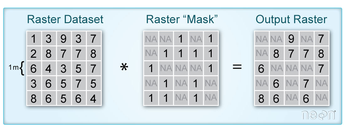
In this tutorial, we demonstrate how to remove parts of a raster based on pixel values using a mask we create. A mask raster layer contains pixel values of either 1 or 0 to where 1 represents pixels that will be used in the analysis and 0 are pixels that are assigned a value of nan (not a number). This can be useful in a number of scenarios, when you are interested in only a certain portion of the data, or need to remove poor-quality data, for example.

import os
import copy
import numpy as np
import numpy.ma as ma
import rasterio as rio
from rasterio.plot import show, show_hist
import requests
import zipfile
import matplotlib.pyplot as plt
from matplotlib import colors
import matplotlib.patches as mpatches
%matplotlib inline

Read in the datasets

Download Lidar Elevation Models and Vegetation Indices from TEAK

To start, we will download the NEON Lidar Aspect and Spectrometer Vegetation Indices (including the NDVI) which are provided in geotiff (.tif) format. Use the download_url function below to download the data directly from the cloud storage location.

# function to download data stored on the internet in a public url to a local file
def download_url(url,download_dir):
    if not os.path.isdir(download_dir):
        os.makedirs(download_dir)
    filename = url.split('/')[-1]
    r = requests.get(url, allow_redirects=True)
    file_object = open(os.path.join(download_dir,filename),'wb')
    file_object.write(r.content)

# define the urls for downloading the Aspect and NDVI geotiff tiles
aspect_url = "https://storage.googleapis.com/neon-aop-products/2021/FullSite/D17/2021_TEAK_5/L3/DiscreteLidar/AspectGtif/NEON_D17_TEAK_DP3_320000_4092000_aspect.tif"
ndvi_url = "https://storage.googleapis.com/neon-aop-products/2021/FullSite/D17/2021_TEAK_5/L3/Spectrometer/VegIndices/NEON_D17_TEAK_DP3_320000_4092000_VegetationIndices.zip"

# download the raster data using the download_url function
download_url(aspect_url,'.\data')
download_url(ndvi_url,'.\data')

# display the contents in the ./data folder to confirm the download completed
os.listdir('./data')

We can use zipfile to unzip the VegetationIndices folder in order to read the NDVI file (which is included in the zipped folder).

with zipfile.ZipFile("./data/NEON_D17_TEAK_DP3_320000_4092000_VegetationIndices.zip","r") as zip_ref:
    zip_ref.extractall("./data")

os.listdir('./data')

Now that the files are downloaded, we can read them in using rasterio.

aspect_file = os.path.join("./data",'NEON_D17_TEAK_DP3_320000_4092000_aspect.tif')
aspect_dataset = rio.open(aspect_file)
aspect_data = aspect_dataset.read(1)

# preview the aspect data
aspect_data

Define and view the spatial extent so we can use this for plotting later on.

ext = [aspect_dataset.bounds.left,
       aspect_dataset.bounds.right,
       aspect_dataset.bounds.bottom,
       aspect_dataset.bounds.top]
ext

Plot the aspect map and histogram.

fig, (ax1, ax2) = plt.subplots(1, 2, figsize=(14,6))
aspect_map = show(aspect_dataset, ax=ax1);
im = aspect_map.get_images()[0]
fig.colorbar(im, label = 'Aspect (degrees)', ax=ax1) # add a colorbar
ax1.ticklabel_format(useOffset=False, style='plain') # turn off scientific notation

show_hist(aspect_dataset, bins=50, histtype='stepfilled',
          lw=0.0, stacked=False, alpha=0.3, ax=ax2);
ax2.set_xlabel("Canopy Height (meters)");
ax2.get_legend().remove()

plt.show();

Classify aspect by direction (North and South)

aspect_reclass = aspect_data.copy()

# classify North and South as 1 & 2
aspect_reclass[np.where(((aspect_data>=0) & (aspect_data<=45)) | (aspect_data>=315))] = 1 #North - Class 1
aspect_reclass[np.where((aspect_data>=135) & (aspect_data<=225))] = 2 #South - Class 2
# West and East are unclassified (nan)
aspect_reclass[np.where(((aspect_data>45) & (aspect_data<135)) | ((aspect_data>225) & (aspect_data<315)))] = np.nan 

Read in the NDVI data to a rasterio dataset.

ndvi_file = os.path.join("./data",'NEON_D17_TEAK_DP3_320000_4092000_NDVI.tif')
ndvi_dataset = rio.open(ndvi_file)
ndvi_data = ndvi_dataset.read(1)

Plot the NDVI map and histogram.

fig, (ax1, ax2) = plt.subplots(1, 2, figsize=(14,6))
ndvi_map = show(ndvi_dataset, cmap = 'RdYlGn', ax=ax1);
im = ndvi_map.get_images()[0]
fig.colorbar(im, label = 'NDVI', ax=ax1) # add a colorbar
ax1.ticklabel_format(useOffset=False, style='plain') # turn off scientific notation

show_hist(ndvi_dataset, bins=50, histtype='stepfilled',
          lw=0.0, stacked=False, alpha=0.3, ax=ax2);
ax2.set_xlabel("NDVI");
ax2.get_legend().remove()

plt.show();

Plot the classified aspect map to highlight the north and south facing slopes.

# Plot classified aspect (N-S) array
fig, ax = plt.subplots(1, 1, figsize=(6,6))
cmap_NS = colors.ListedColormap(['blue','white','red'])
plt.imshow(aspect_reclass,extent=ext,cmap=cmap_NS)
plt.title('TEAK North & South Facing Slopes')
ax=plt.gca(); ax.ticklabel_format(useOffset=False, style='plain') #do not use scientific notation 
rotatexlabels = plt.setp(ax.get_xticklabels(),rotation=90) #rotate x tick labels 90 degrees

# Create custom legend to label N & S
white_box = mpatches.Patch(facecolor='white',label='East, West, or NaN')
blue_box = mpatches.Patch(facecolor='blue', label='North')
red_box = mpatches.Patch(facecolor='red', label='South')
ax.legend(handles=[white_box,blue_box,red_box],handlelength=0.7,bbox_to_anchor=(1.05, 0.45), 
          loc='lower left', borderaxespad=0.);

Mask Data by Aspect and NDVI

Now that we have imported and converted the classified aspect and NDVI rasters to arrays, we can use information from these to find create a new raster consisting of pixels are North facing and have an NDVI > 0.4.

#Mask out pixels that are north facing:
# first make a copy of the ndvi array so we can further select a subset
ndvi_gtpt4 = ndvi_data.copy()
ndvi_gtpt4[ndvi_data<0.4]=np.nan

fig, ax = plt.subplots(1, 1, figsize=(6,6))
plt.imshow(ndvi_gtpt4,extent=ext)
plt.colorbar(); plt.set_cmap('RdYlGn'); 
plt.title('TEAK NDVI > 0.4')
ax=plt.gca(); ax.ticklabel_format(useOffset=False, style='plain') #do not use scientific notation 
rotatexlabels = plt.setp(ax.get_xticklabels(),rotation=90) #rotate x tick labels 90 degrees

#Now include additional requirement that slope is North-facing (i.e. aspectNS_array = 1)
ndvi_gtpt4_north = ndvi_gtpt4.copy()
ndvi_gtpt4_north[aspect_reclass != 1] = np.nan

fig, ax = plt.subplots(1, 1, figsize=(6,6))
plt.imshow(ndvi_gtpt4_north,extent=ext)
plt.colorbar(); plt.set_cmap('RdYlGn'); 
plt.title('TEAK, North Facing & NDVI > 0.4')
ax=plt.gca(); ax.ticklabel_format(useOffset=False, style='plain') #do not use scientific notation 
rotatexlabels = plt.setp(ax.get_xticklabels(),rotation=90) #rotate x tick labels 90 degrees

It looks like there aren't that many parts of the North facing slopes where the NDVI > 0.4. Can you think of why this might be? Hint: consider both ecological reasons and how the flight acquisition might affect NDVI.

Let's also look at where NDVI > 0.4 on south facing slopes.

#Now include additional requirement that slope is Sorth-facing (i.e. aspect_reclass = 2)
ndvi_gtpt4_south = ndvi_gtpt4.copy()
ndvi_gtpt4_south[aspect_reclass != 2] = np.nan

fig, ax = plt.subplots(1, 1, figsize=(6,6))
plt.imshow(ndvi_gtpt4_south,extent=ext)
plt.colorbar(); plt.set_cmap('RdYlGn'); 
plt.title('TEAK, South Facing & NDVI > 0.4')
ax=plt.gca(); ax.ticklabel_format(useOffset=False, style='plain') #do not use scientific notation 
rotatexlabels = plt.setp(ax.get_xticklabels(),rotation=90) #rotate x tick labels 90 degrees

Export Masked Raster to Geotiff

We can also use rasterio to write out the geotiff file. In this case, we will just copy over the metadata from the NDVI raster so that the projection information and everything else is correct. You could create your own metadata dictionary and change the coordinate system, etc. if you chose, but we will keep it simple for this example.

out_meta = ndvi_dataset.meta.copy()
with rio.open('TEAK_NDVIgtpt4_South.tif', 'w', **out_meta) as dst:
    dst.write(ndvi_gtpt4_south, 1)

For peace of mind, let's read back in this raster that we generated and confirm that the contents are identical to the array that we used to generate it. We can do this visually, by plotting it, and also with an equality test.

out_file = "TEAK_NDVIgtpt4_South.tif"
new_dataset = rio.open(out_file)
show(new_dataset);

# use np.array_equal to check that the contents of the file we read back in is the same as the original array 
np.array_equal(new_dataset.read(1),ndvi_gtpt4_south,equal_nan=True)

In this tutorial, we will calculate the biomass for a section of the SJER site. We will be using the Canopy Height Model discrete LiDAR data product as well as NEON field data on vegetation data. This tutorial will calculate biomass for individual trees in the forest.

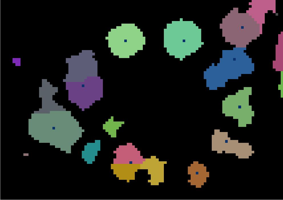
The calculation of biomass consists of four primary steps:

1. Delineate individual tree crowns
2. Calculate predictor variables for all individual trees
3. Collect training data
4. Apply a Random Forest regression model to estimate biomass from the predictor variables

In this tutorial we will use a watershed segmentation algorithm for delineating tree crowns (step 1) and and a Random Forest (RF) machine learning algorithm for relating the predictor variables to biomass (part 4). The predictor variables were selected following suggestions by Gleason et al. (2012) and biomass estimates were determined from DBH (diameter at breast height) measurements following relationships given in Jenkins et al. (2003).

Get Started

First, we will import some Python packages required to run various parts of the script:

import os, sys
import gdal, osr
import numpy as np
import matplotlib.pyplot as plt
from scipy import ndimage as ndi
%matplotlib inline 

Next, we will add libraries from scikit-learn which will help with the watershed delination, determination of predictor variables and random forest algorithm

#Import biomass specific libraries
from skimage.morphology import watershed
from skimage.feature import peak_local_max
from skimage.measure import regionprops
from sklearn.ensemble import RandomForestRegressor

We also need to specify the directory where we will find and save the data needed for this tutorial. You may need to change this line to follow a different working directory structure, or to suit your local machine. I have decided to save my data in the following directory:

data_path = os.path.abspath(os.path.join(os.sep,'neon_biomass_tutorial','data'))
data_path

'D:\\neon_biomass_tutorial\\data'

Define functions

Now we will define a few functions that allow us to more easily work with the NEON data.

• plot_band_array: function to plot NEON geospatial raster data

#Define a function to plot a raster band
def plot_band_array(band_array,image_extent,title,cmap_title,colormap,colormap_limits):
    plt.imshow(band_array,extent=image_extent)
    cbar = plt.colorbar(); plt.set_cmap(colormap); plt.clim(colormap_limits)
    cbar.set_label(cmap_title,rotation=270,labelpad=20)
    plt.title(title); ax = plt.gca()
    ax.ticklabel_format(useOffset=False, style='plain') 
    rotatexlabels = plt.setp(ax.get_xticklabels(),rotation=90)

• array2raster: function to convert a numpy array to a geotiff file

def array2raster(newRasterfn,rasterOrigin,pixelWidth,pixelHeight,array,epsg):

    cols = array.shape[1]
    rows = array.shape[0]
    originX = rasterOrigin[0]
    originY = rasterOrigin[1]

    driver = gdal.GetDriverByName('GTiff')
    outRaster = driver.Create(newRasterfn, cols, rows, 1, gdal.GDT_Float32)
    outRaster.SetGeoTransform((originX, pixelWidth, 0, originY, 0, pixelHeight))
    outband = outRaster.GetRasterBand(1)
    outband.WriteArray(array)
    outRasterSRS = osr.SpatialReference()
    outRasterSRS.ImportFromEPSG(epsg)
    outRaster.SetProjection(outRasterSRS.ExportToWkt())
    outband.FlushCache()

• raster2array: function to conver rasters to an array

def raster2array(geotif_file):
    metadata = {}
    dataset = gdal.Open(geotif_file)
    metadata['array_rows'] = dataset.RasterYSize
    metadata['array_cols'] = dataset.RasterXSize
    metadata['bands'] = dataset.RasterCount
    metadata['driver'] = dataset.GetDriver().LongName
    metadata['projection'] = dataset.GetProjection()
    metadata['geotransform'] = dataset.GetGeoTransform()

    mapinfo = dataset.GetGeoTransform()
    metadata['pixelWidth'] = mapinfo[1]
    metadata['pixelHeight'] = mapinfo[5]

    metadata['ext_dict'] = {}
    metadata['ext_dict']['xMin'] = mapinfo[0]
    metadata['ext_dict']['xMax'] = mapinfo[0] + dataset.RasterXSize/mapinfo[1]
    metadata['ext_dict']['yMin'] = mapinfo[3] + dataset.RasterYSize/mapinfo[5]
    metadata['ext_dict']['yMax'] = mapinfo[3]

    metadata['extent'] = (metadata['ext_dict']['xMin'],metadata['ext_dict']['xMax'],
                          metadata['ext_dict']['yMin'],metadata['ext_dict']['yMax'])

    if metadata['bands'] == 1:
        raster = dataset.GetRasterBand(1)
        metadata['noDataValue'] = raster.GetNoDataValue()
        metadata['scaleFactor'] = raster.GetScale()

        # band statistics
        metadata['bandstats'] = {} # make a nested dictionary to store band stats in same 
        stats = raster.GetStatistics(True,True)
        metadata['bandstats']['min'] = round(stats[0],2)
        metadata['bandstats']['max'] = round(stats[1],2)
        metadata['bandstats']['mean'] = round(stats[2],2)
        metadata['bandstats']['stdev'] = round(stats[3],2)

        array = dataset.GetRasterBand(1).ReadAsArray(0,0,
                                                     metadata['array_cols'],
                                                     metadata['array_rows']).astype(np.float)
        array[array==int(metadata['noDataValue'])]=np.nan
        array = array/metadata['scaleFactor']
        return array, metadata

    else:
        print('More than one band ... function only set up for single band data')

• crown_geometric_volume_pct: function to get the tree height and crown volume percentiles

def crown_geometric_volume_pct(tree_data,min_tree_height,pct):
    p = np.percentile(tree_data, pct)
    tree_data_pct = [v if v < p else p for v in tree_data]
    crown_geometric_volume_pct = np.sum(tree_data_pct - min_tree_height)
    return crown_geometric_volume_pct, p

• get_predictors: function to get the predictor variables from the biomass data

def get_predictors(tree,chm_array, labels):
    indexes_of_tree = np.asarray(np.where(labels==tree.label)).T
    tree_crown_heights = chm_array[indexes_of_tree[:,0],indexes_of_tree[:,1]]
    
    full_crown = np.sum(tree_crown_heights - np.min(tree_crown_heights))
    
    crown50, p50 = crown_geometric_volume_pct(tree_crown_heights,tree.min_intensity,50)
    crown60, p60 = crown_geometric_volume_pct(tree_crown_heights,tree.min_intensity,60)
    crown70, p70 = crown_geometric_volume_pct(tree_crown_heights,tree.min_intensity,70)
        
    return [tree.label,
            np.float(tree.area),
            tree.major_axis_length,
            tree.max_intensity,
            tree.min_intensity, 
            p50, p60, p70,
            full_crown, 
            crown50, crown60, crown70]

Canopy Height Data

With everything set up, we can now start working with our data by define the file path to our CHM file. Note that you will need to change this and subsequent filepaths according to your local machine.

chm_file = os.path.join(data_path,'NEON_D17_SJER_DP3_256000_4106000_CHM.tif')
chm_file

'D:\\neon_biomass_tutorial\\data\\NEON_D17_SJER_DP3_256000_4106000_CHM.tif'

When we output the results, we will want to include the same file information as the input, so we will gather the file name information.

#Get info from chm file for outputting results
chm_name = os.path.basename(chm_file)

Now we will get the CHM data...

chm_array, chm_array_metadata = raster2array(chm_file)

..., plot it, and save the figure.

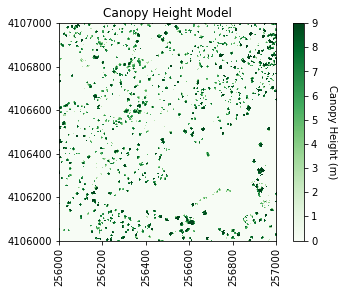
#Plot the original CHM
plt.figure(1)

#Plot the CHM figure
plot_band_array(chm_array,chm_array_metadata['extent'],
                'Canopy Height Model',
                'Canopy Height (m)',
                'Greens',[0, 9])
plt.savefig(os.path.join(data_path,chm_name.replace('.tif','.png')),dpi=300,orientation='landscape',
            bbox_inches='tight',
            pad_inches=0.1)

It looks like SJER primarily has low vegetation with scattered taller trees.

Create Filtered CHM

Now we will use a Gaussian smoothing kernal (convolution) across the data set to remove spurious high vegetation points. This will help ensure we are finding the treetops properly before running the watershed segmentation algorithm.

For different forest types it may be necessary to change the input parameters. Information on the function can be found in the SciPy documentation.

Of most importance are the second and fifth inputs. The second input defines the standard deviation of the Gaussian smoothing kernal. Too large a value will apply too much smoothing, too small and some spurious high points may be left behind. The fifth, the truncate value, controls after how many standard deviations the Gaussian kernal will get cut off (since it theoretically goes to infinity).

#Smooth the CHM using a gaussian filter to remove spurious points
chm_array_smooth = ndi.gaussian_filter(chm_array,2,mode='constant',cval=0,truncate=2.0)
chm_array_smooth[chm_array==0] = 0 

Now save a copy of filtered CHM. We will later use this in our code, so we'll output it into our data directory.

#Save the smoothed CHM
array2raster(os.path.join(data_path,'chm_filter.tif'),
             (chm_array_metadata['ext_dict']['xMin'],chm_array_metadata['ext_dict']['yMax']),
             1,-1,np.array(chm_array_smooth,dtype=float),32611)

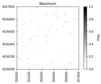
Determine local maximums

Now we will run an algorithm to determine local maximums within the image. Setting indices to False returns a raster of the maximum points, as opposed to a list of coordinates. The footprint parameter is an area where only a single peak can be found. This should be approximately the size of the smallest tree. Information on more sophisticated methods to define the window can be found in Chen (2006).

#Calculate local maximum points in the smoothed CHM
local_maxi = peak_local_max(chm_array_smooth,indices=False, footprint=np.ones((5, 5)))

Our new object local_maxi is an array of boolean values where each pixel is identified as either being the local maximum (True) or not being the local maximum (False).

local_maxi

array([[False, False, False, ..., False, False, False],
       [False, False, False, ..., False, False, False],
       [False, False, False, ..., False, False, False],
       ...,
       [False, False, False, ..., False, False, False],
       [False, False, False, ..., False, False, False],
       [False, False, False, ..., False, False, False]])

This is helpful, but it can be difficult to visualize boolean values using our typical numeric plotting procedures as defined in the plot_band_array function above. Therefore, we will need to convert this boolean array to an numeric format to use this function. Booleans convert easily to integers with values of False=0 and True=1 using the .astype(int) method.

local_maxi.astype(int)

array([[0, 0, 0, ..., 0, 0, 0],
       [0, 0, 0, ..., 0, 0, 0],
       [0, 0, 0, ..., 0, 0, 0],
       ...,
       [0, 0, 0, ..., 0, 0, 0],
       [0, 0, 0, ..., 0, 0, 0],
       [0, 0, 0, ..., 0, 0, 0]])

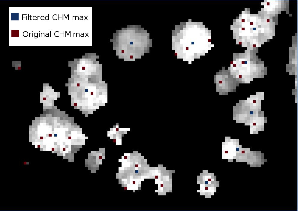
Next we can plot the raster of local maximums by coercing the boolean array into an array of integers inline. The following figure shows the difference in finding local maximums for a filtered vs. non-filtered CHM.

We will save the graphics (.png) in an outputs folder sister to our working directory and data outputs (.tif) to our data directory.

#Plot the local maximums
plt.figure(2)
plot_band_array(local_maxi.astype(int),chm_array_metadata['extent'],
                'Maximum',
                'Maxi',
                'Greys',
                [0, 1])

plt.savefig(data_path+chm_name[0:-4]+ '_Maximums.png',
            dpi=300,orientation='landscape',
            bbox_inches='tight',pad_inches=0.1)

array2raster(data_path+'maximum.tif',
             (chm_array_metadata['ext_dict']['xMin'],chm_array_metadata['ext_dict']['yMax']),
             1,-1,np.array(local_maxi,dtype=np.float32),32611)

If we were to look at the overlap between the tree crowns and the local maxima from each method, it would appear a bit like this raster.

Apply labels to all of the local maximum points

#Identify all the maximum points
markers = ndi.label(local_maxi)[0]

Next we will create a mask layer of all of the vegetation points so that the watershed segmentation will only occur on the trees and not extend into the surrounding ground points. Since 0 represent ground points in the CHM, setting the mask to 1 where the CHM is not zero will define the mask

#Create a CHM mask so the segmentation will only occur on the trees
chm_mask = chm_array_smooth
chm_mask[chm_array_smooth != 0] = 1

Watershed segmentation

As in a river system, a watershed is divided by a ridge that divides areas. Here our watershed are the individual tree canopies and the ridge is the delineation between each one.

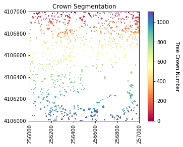
Next, we will perform the watershed segmentation which produces a raster of labels.

#Perform watershed segmentation        
labels = watershed(chm_array_smooth, markers, mask=chm_mask)
labels_for_plot = labels.copy()
labels_for_plot = np.array(labels_for_plot,dtype = np.float32)
labels_for_plot[labels_for_plot==0] = np.nan
max_labels = np.max(labels)

#Plot the segments      
plot_band_array(labels_for_plot,chm_array_metadata['extent'],
                'Crown Segmentation','Tree Crown Number',
                'Spectral',[0, max_labels])

plt.savefig(data_path+chm_name[0:-4]+'_Segmentation.png',
            dpi=300,orientation='landscape',
            bbox_inches='tight',pad_inches=0.1)

array2raster(data_path+'labels.tif',
             (chm_array_metadata['ext_dict']['xMin'],
              chm_array_metadata['ext_dict']['yMax']),
             1,-1,np.array(labels,dtype=float),32611)

Now we will get several properties of the individual trees will be used as predictor variables.

#Get the properties of each segment
tree_properties = regionprops(labels,chm_array)

Now we will get the predictor variables to match the (soon to be loaded) training data using the get_predictors function defined above. The first column will be segment IDs, the rest will be the predictor variables, namely the tree label, area, major_axis_length, maximum height, minimum height, height percentiles (p50, p60, p70), and crown geometric volume percentiles (full and percentiles 50, 60, and 70).

predictors_chm = np.array([get_predictors(tree, chm_array, labels) for tree in tree_properties])
X = predictors_chm[:,1:]
tree_ids = predictors_chm[:,0]

Training data

We now bring in the training data file which is a simple CSV file with no header. If you haven't yet downloaded this, you can scroll up to the top of the lesson and find the Download Data section. The first column is biomass, and the remaining columns are the same predictor variables defined above. The tree diameter and max height are defined in the NEON vegetation structure data along with the tree DBH. The field validated values are used for training, while the other were determined from the CHM and camera images by manually delineating the tree crowns and pulling out the relevant information from the CHM.

Biomass was calculated from DBH according to the formulas in Jenkins et al. (2003).

#Get the full path + training data file
training_data_file = os.path.join(data_path,'SJER_Biomass_Training.csv')

#Read in the training data csv file into a numpy array
training_data = np.genfromtxt(training_data_file,delimiter=',') 

#Grab the biomass (Y) from the first column
biomass = training_data[:,0]

#Grab the biomass predictors from the remaining columns
biomass_predictors = training_data[:,1:12]

Random Forest classifiers

We can then define parameters of the Random Forest classifier and fit the predictor variables from the training data to the Biomass estimates.

#Define parameters for the Random Forest Regressor
max_depth = 30

#Define regressor settings
regr_rf = RandomForestRegressor(max_depth=max_depth, random_state=2)

#Fit the biomass to regressor variables
regr_rf.fit(biomass_predictors,biomass)

RandomForestRegressor(bootstrap=True, ccp_alpha=0.0, criterion='mse',
                      max_depth=30, max_features='auto', max_leaf_nodes=None,
                      max_samples=None, min_impurity_decrease=0.0,
                      min_impurity_split=None, min_samples_leaf=1,
                      min_samples_split=2, min_weight_fraction_leaf=0.0,
                      n_estimators=100, n_jobs=None, oob_score=False,
                      random_state=2, verbose=0, warm_start=False)

We will now apply the Random Forest model to the predictor variables to estimate biomass

#Apply the model to the predictors
estimated_biomass = regr_rf.predict(X)

To output a raster, pre-allocate (copy) an array from the labels raster, then cycle through the segments and assign the biomass estimate to each individual tree segment.

#Set an out raster with the same size as the labels
biomass_map =  np.array((labels),dtype=float)
#Assign the appropriate biomass to the labels
biomass_map[biomass_map==0] = np.nan
for tree_id, biomass_of_tree_id in zip(tree_ids, estimated_biomass):
    biomass_map[biomass_map == tree_id] = biomass_of_tree_id  

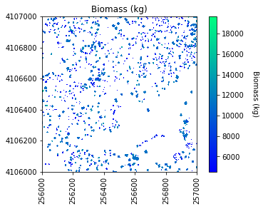
Calculate Biomass

Collect some of the biomass statistics and then plot the results and save an output geotiff.

#Get biomass stats for plotting
mean_biomass = np.mean(estimated_biomass)
std_biomass = np.std(estimated_biomass)
min_biomass = np.min(estimated_biomass)
sum_biomass = np.sum(estimated_biomass)

print('Sum of biomass is ',sum_biomass,' kg')

# Plot the biomass!
plt.figure(5)
plot_band_array(biomass_map,chm_array_metadata['extent'],
                'Biomass (kg)','Biomass (kg)',
                'winter',
                [min_biomass+std_biomass, mean_biomass+std_biomass*3])

# Save the biomass figure; use the same name as the original file, but replace CHM with Biomass
plt.savefig(os.path.join(data_path,chm_name.replace('CHM.tif','Biomass.png')),
            dpi=300,orientation='landscape',
            bbox_inches='tight',
            pad_inches=0.1)

# Use the array2raster function to create a geotiff file of the Biomass
array2raster(os.path.join(data_path,chm_name.replace('CHM.tif','Biomass.tif')),
             (chm_array_metadata['ext_dict']['xMin'],chm_array_metadata['ext_dict']['yMax']),
             1,-1,np.array(biomass_map,dtype=float),32611)

Sum of biomass is  7249752.02745825  kg

This tutorial covers how to create a hillshade from a terrain raster in Python, and demonstrates a few options for visualizing lidar-derived Digital Elevation Models.

First, let's import the required packages:

import os
import numpy as np
import requests
import rasterio as rio
from rasterio.plot import show
import matplotlib.pyplot as plt

Read in the datasets

Download Lidar Elevation Models from TEAK

To start, we will download the NEON Elevation Models (DTM and DSM) which are provided in geotiff (.tif) format. Use the download_url function below to download the data directly from the cloud storage location.

For more information on these data products, refer to the NEON Data Portal page, linked below:

Elevation - LiDAR.

# function to download data stored on the internet in a public url to a local file
def download_url(url,download_dir):
    if not os.path.isdir(download_dir):
        os.makedirs(download_dir)
    filename = url.split('/')[-1]
    r = requests.get(url, allow_redirects=True)
    file_object = open(os.path.join(download_dir,filename),'wb')
    file_object.write(r.content)

# define the urls for downloading the Aspect and NDVI geotiff tiles
dtm_url = "https://storage.googleapis.com/neon-aop-products/2021/FullSite/D17/2021_TEAK_5/L3/DiscreteLidar/DTMGtif/NEON_D17_TEAK_DP3_320000_4092000_DTM.tif"
dsm_url = "https://storage.googleapis.com/neon-aop-products/2021/FullSite/D17/2021_TEAK_5/L3/DiscreteLidar/DSMGtif/NEON_D17_TEAK_DP3_320000_4092000_DSM.tif"

# download the raster data using the download_url function
download_url(dtm_url,'.\data')
download_url(dsm_url,'.\data')

# display the contents in the ./data folder to confirm the download completed
os.listdir('./data')

Calculate Hillshade

Hillshade is used to visualize the hypothetical illumination value (from 0-255) of each pixel on a surface given a specified light source. To calculate hillshade, we need the zenith (altitude) and azimuth of the illumination source, as well as the slope and aspect of the terrain. The formula for hillshade is:

$$Hillshade = 255.0 * (( cos(zenith_I)*cos(slope_T))+(sin(zenith_I)*sin(slope_T)*cos(azimuth_I-aspect_T))$$

Where all angles are in radians.

For more information about how hillshades work, refer to the ESRI ArcGIS page How Hillshade Works.

# function to caluclate hillshade
def hillshade(array,azimuth,angle_altitude):
    azimuth = 360.0 - azimuth 
    
    x, y = np.gradient(array)
    slope = np.pi/2. - np.arctan(np.sqrt(x*x + y*y))
    aspect = np.arctan2(-x, y)
    azm_rad = azimuth*np.pi/180. #azimuth in radians
    alt_rad = angle_altitude*np.pi/180. #altitude in radians
 
    shaded = np.sin(alt_rad)*np.sin(slope) + np.cos(alt_rad)*np.cos(slope)*np.cos((azm_rad - np.pi/2.) - aspect)
    
    return 255*(shaded + 1)/2

dtm_dataset = rio.open(os.path.join('.\data','NEON_D17_TEAK_DP3_320000_4092000_DTM.tif'))
dtm_data = dtm_dataset.read(1)

fig, ax = plt.subplots(1, 1, figsize=(6,6))
dtm_map = show(dtm_dataset,title='Digital Terrain Model',ax=ax);
show(dtm_dataset,contour=True, ax=ax); #overlay the contours
im = dtm_map.get_images()[0]
fig.colorbar(im, label = 'Elevation (m)', ax=ax) # add a colorbar
ax.ticklabel_format(useOffset=False, style='plain') # turn off scientific notation

Now that we have a function to generate hillshade, we need to read in the DTM raster using rasterio and then calculate hillshade using the hillshade function. We can then plot both.

# Use hillshade function on the DTM data array
hs_data = hillshade(dtm_data,225,45)

fig, ax = plt.subplots(1, 1, figsize=(6,6))
ext = [dtm_dataset.bounds.left, dtm_dataset.bounds.right, dtm_dataset.bounds.bottom, dtm_dataset.bounds.top]
plt.imshow(hs_data,extent=ext)
plt.colorbar(); plt.set_cmap('RdYlGn'); 
plt.title('TEAK Hillshade')
ax=plt.gca(); ax.ticklabel_format(useOffset=False, style='plain') #do not use scientific notation 
rotatexlabels = plt.setp(ax.get_xticklabels(),rotation=90) #rotate x tick labels 90 degrees

#Overlay transparent hillshade on DTM:
fig, ax = plt.subplots(1, 1, figsize=(6,6))
im1 = plt.imshow(dtm_data,cmap='terrain_r',extent=ext); 
cbar = plt.colorbar(); cbar.set_label('Elevation, m',rotation=270,labelpad=20)
im2 = plt.imshow(hs_data,cmap='Greys',alpha=0.8,extent=ext); #plt.colorbar()
ax=plt.gca(); ax.ticklabel_format(useOffset=False, style='plain') #do not use scientific notation 
rotatexlabels = plt.setp(ax.get_xticklabels(),rotation=90) #rotate x tick labels 90 degrees
plt.grid('on'); # plt.colorbar(); 
plt.title('TEAK Hillshade + DTM');

Calculate CHM & Overlay on Top of Hillshade

Canopy Height can be simply calculated by subtracting the Digital Terrain Model from the Digital Surface Model. While NEON's CHM is calculated using a slightly more sophisticated "pit-free" algorithm (see the ATBD linked at the top of this tutorial), in this example, we'll calculate the CHM with the simple difference formula. First, read in the DSM data set, which we previously downloaded into the data folder.

dsm_dataset = rio.open(os.path.join('.\data','NEON_D17_TEAK_DP3_320000_4092000_DSM.tif'))
dsm_data = dsm_dataset.read(1)

# calculate CHM by differencing the terrain model (DTM) from the surface model (DSM):
chm_data = dsm_data - dtm_data;

Plot the Canopy Height Model for reference:

fig, ax = plt.subplots(1, 1, figsize=(6,6))
im1 = plt.imshow(chm_data,cmap='Greens',extent=ext); 
ax=plt.gca(); ax.ticklabel_format(useOffset=False, style='plain') #do not use scientific notation 
ax.set_title('Canopy Height Model (DSM-DTM)');

Finally, we can make a plot to bring together all of these visualizations from earlier in the tutorial.

#Overlay transparent hillshade on DTM:
fig, ax = plt.subplots(1, 1, figsize=(10,10))

#Terrain
im1 = plt.imshow(dtm_data,cmap='terrain',extent=ext); 
cbar1 = plt.colorbar(im1,fraction=0.04,pad=0.08,ax=ax); 
cbar1.set_label('Elevation, m',rotation=270,labelpad=20)

#Hillshade
im2 = plt.imshow(hs_data,cmap='Greys',alpha=.5,extent=ext); 

#Canopy
im3 = plt.imshow(chm_data,cmap='Greens',alpha=0.6,extent=ext); 
cbar2 = plt.colorbar(im3,fraction=0.045,pad=0.04,ax=ax); cbar2.set_label('Canopy Height, m',rotation=270,labelpad=15)

ax=plt.gca(); ax.ticklabel_format(useOffset=False, style='plain') #do not use scientific notation 
rotatexlabels = plt.setp(ax.get_xticklabels(),rotation=90) #rotate x tick labels 90 degrees
plt.grid('on'); # plt.colorbar(); 
plt.title('Terrain, Hillshade, & Canopy Height');

This tutorial teaches how to open a NEON AOP HDF5 file with a function, batch processing several HDF5 files, relative comparison between several NIS observations of the same target from different view angles, error checking.

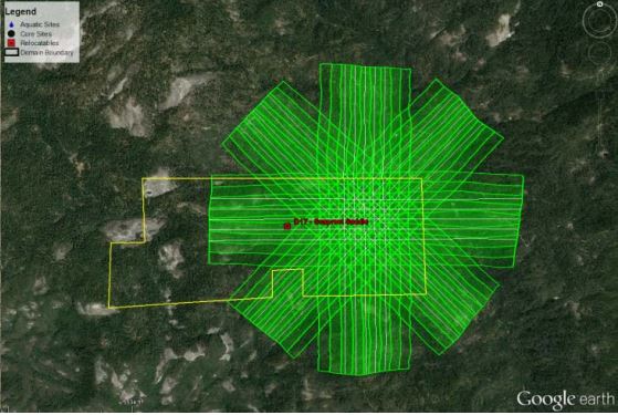
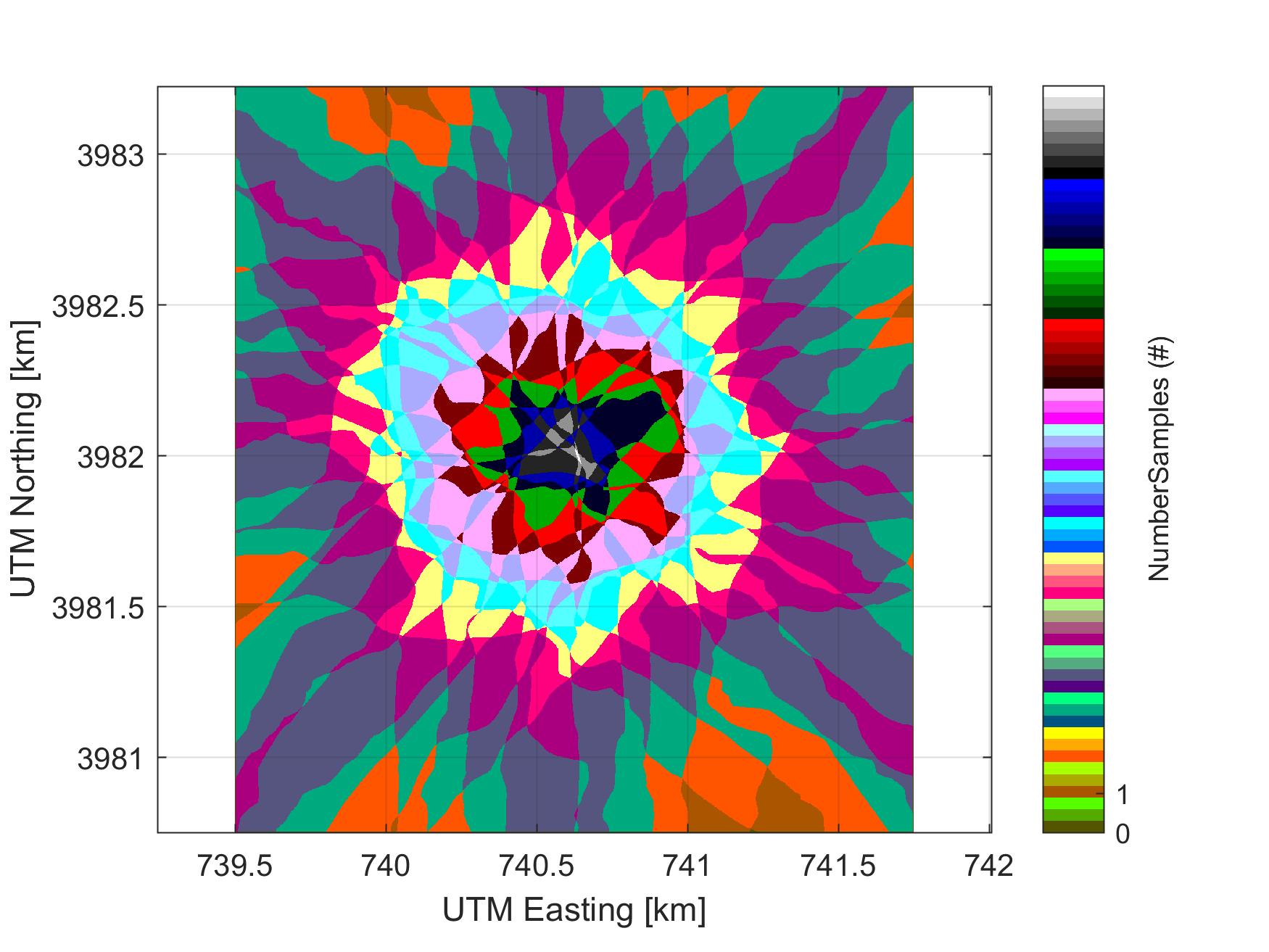
The NEON AOP has flown several special flight plans called BRDF (bi-directional reflectance distribution function) flights. These flights were designed to quantify the the effect of observing targets from a variety of different look-angles, and with varying surface roughness. This allows an assessment of the sensitivity of the NEON imaging spectrometer (NIS) results to these paraemters. THe BRDF flight plan takes the form of a star pattern with repeating overlapping flight lines in each direction. In the center of the pattern is an area where nearly all the flight lines overlap. This area allows us to retrieve a reflectance curve of the same targat from the many different flight lines to visualize how then change for each acquisition. The following figure displays a BRDF flight plan as well as the number of flightlines (samples) which are overlapping.

To date (June 2017), the NEON AOP has flown a BRDF flight at SJER and SOAP (D17) and ORNL (D07). We will work with the ORNL BRDF flight and retrieve reflectance curves from up to 18 lines and compare them to visualize the differences in the resulting curves. To reduce the file size, each of the BRDF flight lines have been reduced to a rectangular area covering where all lines are overlapping, additionally several of the ancillary rasters normally included have been removed in order to reduce file size.

We'll start off by again adding necessary libraries and our NEON AOP HDF5 reader function.

import h5py
import csv
import numpy as np
import os
import gdal
import matplotlib.pyplot as plt
import sys
from math import floor
import time
import warnings
warnings.filterwarnings('ignore')

def h5refl2array(h5_filename):
    hdf5_file = h5py.File(h5_filename,'r')

    #Get the site name
    file_attrs_string = str(list(hdf5_file.items()))
    file_attrs_string_split = file_attrs_string.split("'")
    sitename = file_attrs_string_split[1]
    refl = hdf5_file[sitename]['Reflectance']
    reflArray = refl['Reflectance_Data']
    refl_shape = reflArray.shape
    wavelengths = refl['Metadata']['Spectral_Data']['Wavelength']
    #Create dictionary containing relevant metadata information
    metadata = {}
    metadata['shape'] = reflArray.shape
    metadata['mapInfo'] = refl['Metadata']['Coordinate_System']['Map_Info']
    #Extract no data value & set no data value to NaN\n",
    metadata['scaleFactor'] = float(reflArray.attrs['Scale_Factor'])
    metadata['noDataVal'] = float(reflArray.attrs['Data_Ignore_Value'])
    metadata['bad_band_window1'] = (refl.attrs['Band_Window_1_Nanometers'])
    metadata['bad_band_window2'] = (refl.attrs['Band_Window_2_Nanometers'])
    metadata['projection'] = refl['Metadata']['Coordinate_System']['Proj4'].value
    metadata['EPSG'] = int(refl['Metadata']['Coordinate_System']['EPSG Code'].value)
    mapInfo = refl['Metadata']['Coordinate_System']['Map_Info'].value
    mapInfo_string = str(mapInfo); #print('Map Info:',mapInfo_string)\n",
    mapInfo_split = mapInfo_string.split(",")
    #Extract the resolution & convert to floating decimal number
    metadata['res'] = {}
    metadata['res']['pixelWidth'] = mapInfo_split[5]
    metadata['res']['pixelHeight'] = mapInfo_split[6]
    #Extract the upper left-hand corner coordinates from mapInfo\n",
    xMin = float(mapInfo_split[3]) #convert from string to floating point number\n",
    yMax = float(mapInfo_split[4])
    #Calculate the xMax and yMin values from the dimensions\n",
    xMax = xMin + (refl_shape[1]*float(metadata['res']['pixelWidth'])) #xMax = left edge + (# of columns * resolution)\n",
    yMin = yMax - (refl_shape[0]*float(metadata['res']['pixelHeight'])) #yMin = top edge - (# of rows * resolution)\n",
    metadata['extent'] = (xMin,xMax,yMin,yMax),
    metadata['ext_dict'] = {}
    metadata['ext_dict']['xMin'] = xMin
    metadata['ext_dict']['xMax'] = xMax
    metadata['ext_dict']['yMin'] = yMin
    metadata['ext_dict']['yMax'] = yMax
    hdf5_file.close        
    return reflArray, metadata, wavelengths

print('Starting BRDF Analysis')

Starting BRDF Analysis

First we will define the extents of the rectangular array containing the section from each BRDF flightline.

BRDF_rectangle = np.array([[740315,3982265],[740928,3981839]],np.float)

Next we will define the coordinates of the target of interest. These can be set as any coordinate pait that falls within the rectangle above, therefore the coordaintes must be in UTM Zone 16 N.

x_coord = 740600
y_coord = 3982000

To prevent the function of failing, we will first check to ensure the coordinates are within the rectangular bounding box. If they are not, we throw an error message and exit from the script.

if BRDF_rectangle[0,0] <= x_coord <= BRDF_rectangle[1,0] and BRDF_rectangle[1,1] <= y_coord <= BRDF_rectangle[0,1]:
    print('Point in bounding area')
    y_index = floor(x_coord - BRDF_rectangle[0,0])
    x_index = floor(BRDF_rectangle[0,1] - y_coord)
else:
    print('Point not in bounding area, exiting')
    raise Exception('exit')

Point in bounding area

Now we will define the location of the all the subset NEON AOP h5 files from the BRDF flight

## You will need to update this filepath for your local data directory
h5_directory = "/Users/olearyd/Git/data/F07A/"

Now we will grab all files / folders within the defined directory and then cycle through them and retain only the h5files

files = os.listdir(h5_directory)
h5_files = [i for i in files if i.endswith('.h5')]

Now we will print the h5 files to make sure they have been included and set up a figure for plotting all of the reflectance curves

print(h5_files)

fig=plt.figure()
ax = plt.subplot(111)

['NEON_D07_F07A_DP1_20160611_162007_reflectance_modify.h5', 'NEON_D07_F07A_DP1_20160611_172430_reflectance_modify.h5', 'NEON_D07_F07A_DP1_20160611_170118_reflectance_modify.h5', 'NEON_D07_F07A_DP1_20160611_164259_reflectance_modify.h5', 'NEON_D07_F07A_DP1_20160611_171403_reflectance_modify.h5', 'NEON_D07_F07A_DP1_20160611_160846_reflectance_modify.h5', 'NEON_D07_F07A_DP1_20160611_170922_reflectance_modify.h5', 'NEON_D07_F07A_DP1_20160611_162514_reflectance_modify.h5', 'NEON_D07_F07A_DP1_20160611_160444_reflectance_modify.h5', 'NEON_D07_F07A_DP1_20160611_170538_reflectance_modify.h5', 'NEON_D07_F07A_DP1_20160611_171852_reflectance_modify.h5', 'NEON_D07_F07A_DP1_20160611_163945_reflectance_modify.h5', 'NEON_D07_F07A_DP1_20160611_163424_reflectance_modify.h5', 'NEON_D07_F07A_DP1_20160611_165240_reflectance_modify.h5', 'NEON_D07_F07A_DP1_20160611_161228_reflectance_modify.h5', 'NEON_D07_F07A_DP1_20160611_162951_reflectance_modify.h5', 'NEON_D07_F07A_DP1_20160611_161532_reflectance_modify.h5', 'NEON_D07_F07A_DP1_20160611_165711_reflectance_modify.h5', 'NEON_D07_F07A_DP1_20160611_164809_reflectance_modify.h5']

Now we will begin cycling through all of the h5 files and retrieving the information we need also print the file that is currently being processed

Inside the for loop we will

1. read in the reflectance data and the associated metadata, but construct the file name from the generated file list

2. Determine the indexes of the water vapor bands (bad band windows) in order to mask out all of the bad bands

3. Read in the reflectance dataset using the NEON AOP H5 reader function

4. Check the first value the first value of the reflectance curve (actually any value). If it is equivalent to the NO DATA value, then coordainte chosen did not intersect a pixel for the flight line. We will just continue and move to the next line.

5. Apply NaN values to the areas contianing the bad bands

6. Split the contents of the file name so we can get the line number for labelling in the plot.

7. Plot the curve

for file in h5_files:

    print('Working on ' + file)
    
    [reflArray,metadata,wavelengths] = h5refl2array(h5_directory+file)
    bad_band_window1 = (metadata['bad_band_window1'])
    bad_band_window2 = (metadata['bad_band_window2'])

    index_bad_window1 = [i for i, x in enumerate(wavelengths) if x > bad_band_window1[0] and x < bad_band_window1[1]]
    index_bad_window2 = [i for i, x in enumerate(wavelengths) if x > bad_band_window2[0] and x < bad_band_window2[1]]
    
    index_bad_windows = index_bad_window1+index_bad_window2
    reflectance_curve = np.asarray(reflArray[y_index,x_index,:], dtype=np.float32)
    if reflectance_curve[0] == metadata['noDataVal']:
        continue
    reflectance_curve[index_bad_windows] = np.nan
    filename_split = (file).split("_") 
    ax.plot(wavelengths,reflectance_curve/metadata['scaleFactor'],label = filename_split[5]+' Reflectance')

Working on NEON_D07_F07A_DP1_20160611_162007_reflectance_modify.h5
Working on NEON_D07_F07A_DP1_20160611_172430_reflectance_modify.h5
Working on NEON_D07_F07A_DP1_20160611_170118_reflectance_modify.h5
Working on NEON_D07_F07A_DP1_20160611_164259_reflectance_modify.h5
Working on NEON_D07_F07A_DP1_20160611_171403_reflectance_modify.h5
Working on NEON_D07_F07A_DP1_20160611_160846_reflectance_modify.h5
Working on NEON_D07_F07A_DP1_20160611_170922_reflectance_modify.h5
Working on NEON_D07_F07A_DP1_20160611_162514_reflectance_modify.h5
Working on NEON_D07_F07A_DP1_20160611_160444_reflectance_modify.h5
Working on NEON_D07_F07A_DP1_20160611_170538_reflectance_modify.h5
Working on NEON_D07_F07A_DP1_20160611_171852_reflectance_modify.h5
Working on NEON_D07_F07A_DP1_20160611_163945_reflectance_modify.h5
Working on NEON_D07_F07A_DP1_20160611_163424_reflectance_modify.h5
Working on NEON_D07_F07A_DP1_20160611_165240_reflectance_modify.h5
Working on NEON_D07_F07A_DP1_20160611_161228_reflectance_modify.h5
Working on NEON_D07_F07A_DP1_20160611_162951_reflectance_modify.h5
Working on NEON_D07_F07A_DP1_20160611_161532_reflectance_modify.h5
Working on NEON_D07_F07A_DP1_20160611_165711_reflectance_modify.h5
Working on NEON_D07_F07A_DP1_20160611_164809_reflectance_modify.h5

This plots the reflectance curves from all lines onto the same plot. Now, we will add the appropriate legend and plot labels, display and save the plot with the coordaintes in the file name so we can repeat the position of the target

box = ax.get_position()
ax.set_position([box.x0, box.y0, box.width * 0.8, box.height])
ax.legend(loc='center left',bbox_to_anchor=(1,0.5))
plt.title('BRDF Reflectance Curves at ' + str(x_coord) +' '+ str(y_coord))
plt.xlabel('Wavelength (nm)'); plt.ylabel('Refelctance (%)')
fig.savefig('BRDF_uncertainty_at_' + str(x_coord) +'_'+ str(y_coord)+'.png',dpi=500,orientation='landscape',bbox_inches='tight',pad_inches=0.1)
plt.show()

It is possible that the figure above does not display properly, which is why we use the fig.save() method above to store the resulting figure as its own PNG file in the same directory as this Jupyter Notebook file.

The result is a plot with all the curves in which we can visualize the difference in the observations simply by chaging the flight direction with repect to the ground target.

Experiment with changing the coordinates to analyze different targets within the rectangle.

In this tutorial we will learn how to retrieve reflectance curves from a pre-specified coordinate in a NEON AOP HDF5 file, retrieve bad band window indexes and mask portions of a reflectance curve, plot reflectance curves, and gain an understanding of some sources of uncertainty in Neon Imaging Spectrometer (NIS) data.

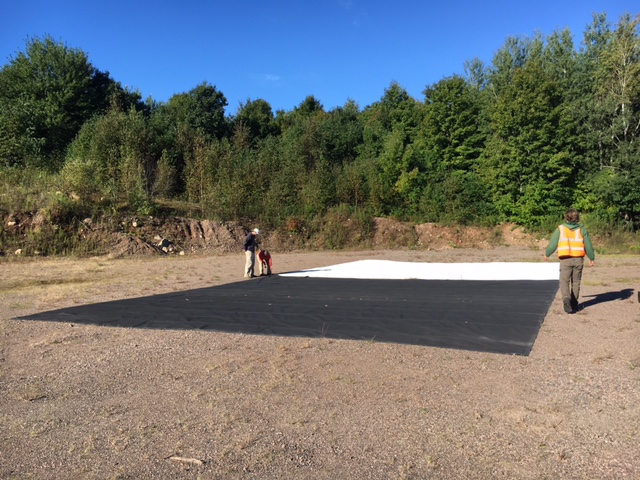
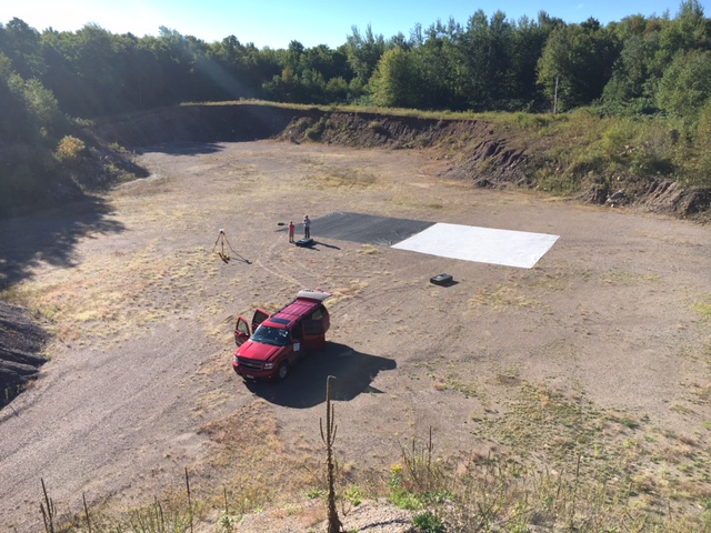
In this tutorial we will be examining the accuracy of the Neon Imaging Spectrometer (NIS) against targets with known reflectance values. The targets consist of two 10 x 10 m tarps which have been specially designed to have 3% reflectance (black tarp) and 48% reflectance (white tarp) across all of the wavelengths collected by the NIS (see images below). During the Sept. 12 2016 flight over the Chequamegon-Nicolet National Forest (CHEQ), an area in D05 which is part of NEON's Steigerwaldt (STEI) site, these tarps were deployed in a gravel pit. During the airborne overflight, observations were also taken over the tarps with an Analytical Spectral Device (ASD), which is a hand-held field spectrometer. The ASD measurements provide a validation source against the airborne measurements.

To test the accuracy, we will plot reflectance curves from the ASD measurments over the spectral tarps as well as reflectance curves from the NIS over the associated flight line. We can then carry out absolute and relative comparisons. The major error sources in the NIS can be generally categorized into the following components:

1. Calibration of the sensor
2. Quality of ortho-rectification
3. Accuracy of radiative transfer code and subsequent ATCOR interpolation
4. Selection of atmospheric input parameters
5. Terrain relief
6. Terrain cover

Note that ATCOR (the atmospheric correction software used by AOP) specifies the accuracy of reflectance retrievals to be between 3 and 5% of total reflectance. The tarps are located in a flat area, therefore, influences by terrain relief should be minimal. We will have to keep the remining errors in mind as we analyze the data.

Get Started

We'll start by importing all of the necessary packages to run the Python script.

import os, sys
import numpy as np
import requests
import h5py
import csv
import gdal
import matplotlib.pyplot as plt
%matplotlib inline

Define a function to read the hdf5 reflectance files and associated metadata into Python:

def h5refl2array(h5_filename):
    hdf5_file = h5py.File(h5_filename,'r')

    #Get the site name
    file_attrs_string = str(list(hdf5_file.items()))
    file_attrs_string_split = file_attrs_string.split("'")
    sitename = file_attrs_string_split[1]
    refl = hdf5_file[sitename]['Reflectance']
    reflArray = refl['Reflectance_Data']
    refl_shape = reflArray.shape
    wavelengths = refl['Metadata']['Spectral_Data']['Wavelength']
    #Create dictionary containing relevant metadata information
    metadata = {}
    metadata['shape'] = reflArray.shape
    metadata['mapInfo'] = refl['Metadata']['Coordinate_System']['Map_Info']
    #Extract no data value & set no data value to NaN\n",
    metadata['scaleFactor'] = float(reflArray.attrs['Scale_Factor'])
    metadata['noDataVal'] = float(reflArray.attrs['Data_Ignore_Value'])
    metadata['bad_band_window1'] = (refl.attrs['Band_Window_1_Nanometers'])
    metadata['bad_band_window2'] = (refl.attrs['Band_Window_2_Nanometers'])
    metadata['projection'] = refl['Metadata']['Coordinate_System']['Proj4'][()]
    metadata['EPSG'] = int(refl['Metadata']['Coordinate_System']['EPSG Code'][()])
    mapInfo = refl['Metadata']['Coordinate_System']['Map_Info'][()]
    mapInfo_string = str(mapInfo); #print('Map Info:',mapInfo_string)\n",
    mapInfo_split = mapInfo_string.split(",")
    #Extract the resolution & convert to floating decimal number
    metadata['res'] = {}
    metadata['res']['pixelWidth'] = mapInfo_split[5]
    metadata['res']['pixelHeight'] = mapInfo_split[6]
    #Extract the upper left-hand corner coordinates from mapInfo\n",
    xMin = float(mapInfo_split[3]) #convert from string to floating point number\n",
    yMax = float(mapInfo_split[4])
    #Calculate the xMax and yMin values from the dimensions\n",
    xMax = xMin + (refl_shape[1]*float(metadata['res']['pixelWidth'])) #xMax = left edge + (# of columns * resolution)\n",
    yMin = yMax - (refl_shape[0]*float(metadata['res']['pixelHeight'])) #yMin = top edge - (# of rows * resolution)\n",
    metadata['extent'] = (xMin,xMax,yMin,yMax),
    metadata['ext_dict'] = {}
    metadata['ext_dict']['xMin'] = xMin
    metadata['ext_dict']['xMax'] = xMax
    metadata['ext_dict']['yMin'] = yMin
    metadata['ext_dict']['yMax'] = yMax
    hdf5_file.close        
    return reflArray, metadata, wavelengths

Set up the directory where you are storing the data for this lesson. The variable h5_filename is the flightline which covers the tarps. Save the h5 file which you downloaded (see the Download Data instructions at the beginning of the tutorial) to your working directory. For this lesson we've set up a subfolder './data' in the current working directory to save all the data. You can save it elsewhere, but just need to update your code to point to the correct directory.

## You will need to change these filepaths according to how you've set up your directory
## As you can see here, I saved the files downloaded above into a sub-directory named "./data"
h5_filename = r'./data/NEON_D05_CHEQ_DP1_20160912_160540_reflectance.h5'

Define a function that will read in the contents of a url and write it out to a file:

def url_to_file(url,outfile):
    response = requests.get(url)
    open(outfile,"wb").write(response.content)

Run the function on the two urls where the ASD reflectance data is saved, in the NEON-Data-Skills GitHub repository for this lesson.

tarp_03_url = "https://raw.githubusercontent.com/NEONScience/NEON-Data-Skills/main/tutorials/Python/Hyperspectral/uncertainty-and-validation/hyperspectral_validation_py/data/CHEQ_Tarp_03_02_refl_bavg.txt"
tarp_48_url = "https://raw.githubusercontent.com/NEONScience/NEON-Data-Skills/main/tutorials/Python/Hyperspectral/uncertainty-and-validation/hyperspectral_validation_py/data/CHEQ_Tarp_48_01_refl_bavg.txt"

url_to_file(tarp_48_url,'./data/CHEQ_Tarp_48_01_refl_bavg.txt')
url_to_file(tarp_03_url,'./data/CHEQ_Tarp_03_02_refl_bavg.txt')

We can now set the path to these files. The files read into the variables tarp_48_filename and tarp_03_filename contain the field validated spectra for the white and black tarp respectively, organized by wavelength and reflectance.

tarp_48_filename = r'./data/CHEQ_Tarp_48_01_refl_bavg.txt'
tarp_03_filename = r'./data/CHEQ_Tarp_03_02_refl_bavg.txt'

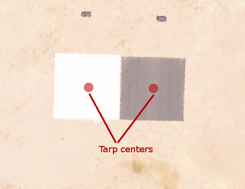
We want to pull the spectra from the airborne data from the center of the tarp to minimize any errors introduced by infiltrating light in adjacent pixels, or through errors in ortho-rectification (source 2). We have pre-determined the coordinates for the center of each tarp which are as follows:

48% reflectance tarp UTMx: 727487, UTMy: 5078970

3% reflectance tarp UTMx: 727497, UTMy: 5078970

Let's define these coordinates:

tarp_48_center = np.array([727487,5078970])
tarp_03_center = np.array([727497,5078970])

Now we'll use our function designed for NEON AOP's HDF5 files to access the hyperspectral data

[reflArray,metadata,wavelengths] = h5refl2array(h5_filename)

Within the reflectance curves there are areas with noisy data due to atmospheric windows in the water absorption bands. For this exercise we do not want to plot these areas as they obscure details in the plots due to their anomolous values. The metadata associated with these band locations is contained in the metadata gathered by our function. We will pull out these areas as 'bad band windows' and determine which indexes in the reflectance curves encompass these bad bands.

bad_band_window1 = (metadata['bad_band_window1'])
bad_band_window2 = (metadata['bad_band_window2'])

index_bad_window1 = [i for i, x in enumerate(wavelengths) if x > bad_band_window1[0] and x < bad_band_window1[1]]
index_bad_window2 = [i for i, x in enumerate(wavelengths) if x > bad_band_window2[0] and x < bad_band_window2[1]]

# join the lists of indexes into a single variable
index_bad_windows = index_bad_window1 + index_bad_window2

The reflectance data is saved in files which are 'tab delimited.' We will use a numpy function np.genfromtxt to read in the tarp reflectance data observed with the ASD using the tab ('\t') delimiter.

tarp_48_data = np.genfromtxt(tarp_48_filename, delimiter = '\t')
tarp_03_data = np.genfromtxt(tarp_03_filename, delimiter = '\t')

Now we'll set all the data inside of the bad band windows to NaNs (not a number) so they will not be included in the plots.

tarp_48_data[index_bad_windows] = np.nan
tarp_03_data[index_bad_windows] = np.nan

The next step is to determine which pixel in the reflectance data belongs to the center of each tarp. To do this, we will subtract the tarp center pixel location from the upper left corner pixels specified in the map info of the H5 file. This information is saved in the metadata dictionary output from our function that reads NEON AOP HDF5 files. The difference between these coordinates gives us the x and y index of the reflectance curve.

x_tarp_48_index = int((tarp_48_center[0] - metadata['ext_dict']['xMin'])/float(metadata['res']['pixelWidth']))
y_tarp_48_index = int((metadata['ext_dict']['yMax'] - tarp_48_center[1])/float(metadata['res']['pixelHeight']))

x_tarp_03_index = int((tarp_03_center[0] - metadata['ext_dict']['xMin'])/float(metadata['res']['pixelWidth']))
y_tarp_03_index = int((metadata['ext_dict']['yMax'] - tarp_03_center[1])/float(metadata['res']['pixelHeight']))

Next, we will plot both the curve from the airborne data taken at the center of the tarps as well as the curves obtained from the ASD data to provide a visualization of their consistency for both tarps. Once generated, we will also save the figure to a pre-determined location.

plt.figure(1)
tarp_48_reflectance = np.asarray(reflArray[y_tarp_48_index,x_tarp_48_index,:], dtype=np.float32)/metadata['scaleFactor']
tarp_48_reflectance[index_bad_windows] = np.nan
plt.plot(wavelengths,tarp_48_reflectance,label = 'Airborne Reflectance')
plt.plot(wavelengths,tarp_48_data[:,1], label = 'ASD Reflectance')
plt.title('CHEQ 20160912 48% tarp')
plt.xlabel('Wavelength (nm)'); plt.ylabel('Reflectance (%)')
plt.legend()
#plt.savefig('CHEQ_20160912_48_tarp.png',dpi=300,orientation='landscape',bbox_inches='tight',pad_inches=0.1)

plt.figure(2)
tarp_03_reflectance = np.asarray(reflArray[y_tarp_03_index,x_tarp_03_index,:], dtype=np.float32)/ metadata['scaleFactor']
tarp_03_reflectance[index_bad_windows] = np.nan
plt.plot(wavelengths,tarp_03_reflectance,label = 'Airborne Reflectance')
plt.plot(wavelengths,tarp_03_data[:,1],label = 'ASD Reflectance')
plt.title('CHEQ 20160912 3% tarp')
plt.xlabel('Wavelength (nm)'); plt.ylabel('Reflectance (%)')
plt.legend();
#plt.savefig('CHEQ_20160912_3_tarp.png',dpi=300,orientation='landscape',bbox_inches='tight',pad_inches=0.1)

This produces plots showing the results of the ASD and airborne measurements over the 48% tarp. Visually, the comparison between the two appears to be fairly good. However, over the 3% tarp we appear to be over-estimating the reflectance. Large absolute differences could be associated with ATCOR input parameters (source 4). For example, the user must input the local visibility, which is related to aerosol optical thickness (AOT). We don't measure this at every site, therefore input a standard parameter for all sites.

Given the 3% reflectance tarp has much lower overall reflectance, it may be more informative to determine what the absolute difference between the two curves are and plot that as well.

plt.figure(3)
plt.plot(wavelengths,tarp_48_reflectance-tarp_48_data[:,1])
plt.title('CHEQ 20160912 48% tarp absolute difference')
plt.xlabel('Wavelength (nm)'); plt.ylabel('Absolute Reflectance Difference (%)')
#plt.savefig('CHEQ_20160912_48_tarp_absolute_diff.png',dpi=300,orientation='landscape',bbox_inches='tight',pad_inches=0.1)

plt.figure(4)
plt.plot(wavelengths,tarp_03_reflectance-tarp_03_data[:,1])
plt.title('CHEQ 20160912 3% tarp absolute difference')
plt.xlabel('Wavelength (nm)'); plt.ylabel('Absolute Reflectance Difference (%)');
#plt.savefig('CHEQ_20160912_3_tarp_absolute_diff.png',dpi=300,orientation='landscape',bbox_inches='tight',pad_inches=0.1)

From this we are able to see that the 48% tarp actually has larger absolute differences than the 3% tarp. The 48% tarp performs poorly at the shortest and longest wavelenghths as well as near the edges of the bad band windows. This is related to difficulty in calibrating the sensor in these sensitive areas.

Let's now determine the result of the percent difference, which is the metric used by ATCOR to report accuracy. We can do this by calculating the ratio of the absolute difference between curves to the total reflectance

plt.figure(5)
relative_diff_48 = 100*(np.divide(tarp_48_reflectance-tarp_48_data[:,1],tarp_48_data[:,1]))
plt.plot(wavelengths,100*np.divide(tarp_48_reflectance-tarp_48_data[:,1],tarp_48_data[:,1]));
plt.title('CHEQ 20160912 48% tarp percent difference')
plt.xlabel('Wavelength (nm)'); plt.ylabel('Percent Reflectance Difference')
plt.ylim((-100,100))
#plt.savefig('CHEQ_20160912_48_tarp_relative_diff.png',dpi=300,orientation='landscape',bbox_inches='tight',pad_inches=0.1)

plt.figure(6)
plt.plot(wavelengths,100*np.divide(tarp_03_reflectance-tarp_03_data[:,1],tarp_03_data[:,1]));
plt.title('CHEQ 20160912 3% tarp percent difference')
plt.xlabel('Wavelength (nm)'); plt.ylabel('Percent Reflectance Difference')
plt.ylim((-100,150));
#plt.savefig('CHEQ_20160912_3_tarp_relative_diff.png',dpi=300,orientation='landscape',bbox_inches='tight',pad_inches=0.1)

From these plots we can see that even though the absolute error on the 48% tarp was larger, the relative error on the 48% tarp is generally much smaller. The 3% tarp can have errors exceeding 50% for most of the tarp. This indicates that targets with low reflectance values may have higher relative errors.

This tutorial covers how to set up a Central Repo as a remote to your local repo in order to update your local fork with updates. You want to do this every time before starting new edits in your local repo.

We now have done the following:

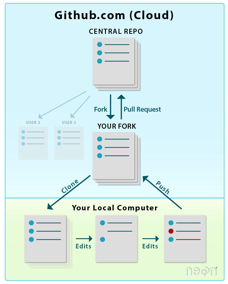
1. We've forked (made an individual copy of) the NEONScience/DI-NEON-participants repo to our github.com account.
2. We've cloned the forked repo - making a copy of it on our local computers.
3. We've added files and content to our local copy of the repo and committed the changes.
4. We've pushed those changes back up to our forked repo on github.com.
5. We've completed a Pull Request to update the central repository with our changes.

Once you're all setup to work on your project, you won't need to repeat the fork and clone steps. But you do want to update your local repository with any changes other's may have added to the central repository. How do we do this?

We will do this by directly pulling the updates from the central repo to our local repo by setting up the local repo as a "remote". A "remote" repo is any repo which is not the repo that you are currently working in.

Update, then Work

Once you've established working in your repo, you should follow these steps when starting to work each time in the repo:

1. Update your local repo from the central repo (git pull upstream master).
2. Make edits, save, git add, and git commit all in your local repo.
3. Push changes from local repo to your fork on github.com (git push origin master)
4. Update the central repo from your fork (Pull Request)
5. Repeat.

Notice that we've already learned how to do steps 2-4, now we are completing the circle by learning to update our local repo directly with any changes from the central repo.

The order of steps above is important as it ensures that you incorporate any changes that have been made to the NEON central repository into your forked & local repos prior to adding changes to the central repo. If you do not sync in this order, you are at greater risk of creating a merge conflict.

What's A Merge Conflict?

A merge conflict occurs when two users edit the same part of a file at the same time. Git cannot decide which edit was first and which was last, and therefore which edit should be in the most current copy. Hence the conflict.

Set up Upstream Remote

We want to directly update our local repo with any changes made in the central repo prior to starting our next edits or additions. To do this we need to set up the central repository as an upstream remote for our repo.

Step 1: Get Central Repository URL

First, we need the URL of the central repository. Navigate to the central repository in GitHub NEONScience/DI-NEON-participants. Select the green Clone or Download button (just like we did when we cloned the repo) to copy the URL of the repo.

Step 2: Add the Remote

Second, we need to connect the upstream remote -- the central repository to our local repo.

Make sure you are still in you local repository in bash

First, navigate to the desired directory.

$ cd ~/Documents/GitHub/DI-NEON-participants

and then type:

$ git remote add upstream https://github.com/NEONScience/DI-NEON-participants.git

Here you are identifying that is is a git command with git and then that you are adding an upstream remote with the given URL.

Step 3: Update Local Repo

Use git pull to sync your local repo with the forked GitHub.com repo.

Second, update local repo using git pull with the added directions of upstream indicating the central repository and master specifying which branch you are pulling down (remember, branches are a great tool to look into once you're comfortable with Git and GitHub, but we aren't going to focus on them. Just use master).

$ git pull upstream master

remote: Counting objects: 25, done.
remote: Compressing objects: 100% (15/15), done.
remote: Total 25 (delta 16), reused 19 (delta 10), pack-reused 0
Unpacking objects: 100% (25/25), done.
From https://github.com/NEONScience/DI-NEON-participants
    74d9b7b..463e6f0  master   -> origin/master
Auto-merging _posts/institute-materials/example.md

Understand the output: The output will change with every update, several things to look for in the output:

• remote: …: tells you how many items have changed.
• From https:URL: which remote repository is data being pulled from. We set up the central repository as the remote but it can be lots of other repos too.
• Section with + and - : this visually shows you which documents are updated and the types of edits (additions/deletions) that were made.

Now that you've synced your local repo, let's check the status of the repo.

$ git status

Step 4: Complete the Cycle

Now you are set up with the additions, you will need to add and commit those changes. Once you've done that, you can push the changes back up to your fork on github.com.

$ git push origin master

Now your commits are added to your forked repo on github.com and you're ready to repeat the loop with a Pull Request.

Workflow Summary

Syncing Central Repo with Local Repo

Setting It Up (only do this the initial time)

• Find & copy Central Repo URL
• git remote add upstream https://github.com/NEONScience/DI-NEON-participants.git

After Initial Set Up

• Update your Local Repo & Push Changes

  • git pull upstream master - pull down any changes and sync the local repo with the central repo
  • make changes, git add and git commit
  • git push origin master - push your changes up to your fork
  • Repeat

  ---

  Have questions? No problem. Leave your question in the comment box below. It's likely some of your colleagues have the same question, too! And also likely someone else knows the answer.

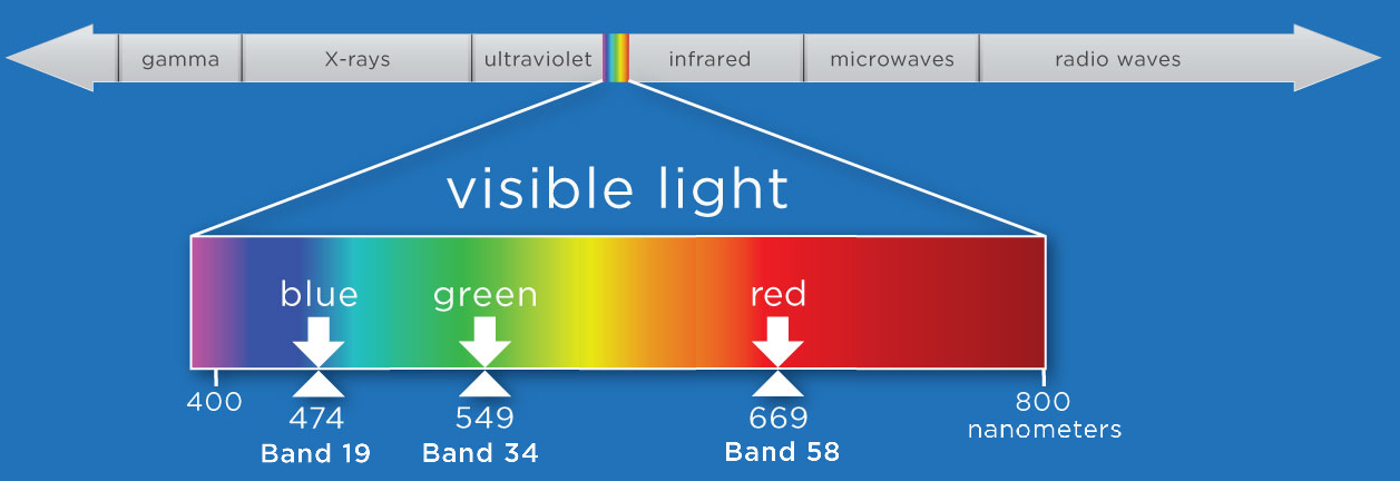
In this tutorial, you will learn how to efficiently read in hyperspectral surface directional reflectance hdf5 data and metadata, plot a single band and Red-Green-Blue (RGB) band combinations of a reflectance data tile using Python functions created for working with and visualizing NEON AOP hyperspectral data.

This tutorial works with the Level 3 Spectrometer orthorectified surface directional reflectance - mosaic data product.

We can combine any three bands from the NEON reflectance data to make an RGB image that will depict different information about the Earth's surface. A natural color image, made with bands from the red, green, and blue wavelengths looks close to what we would see with the naked eye. We can also choose band combinations from other wavelenghts, and map them to the red, blue, and green colors to highlight different features. A false color image is made with one or more bands from a non-visible portion of the electromagnetic spectrum that are mapped to red, green, and blue colors. These images can display other information about the landscape that is not easily seen with a natural color image.

The NASA Goddard Media Studio video "Peeling Back Landsat's Layers of Data" gives a good quick overview of natural and false color band combinations. Note that the Landsat multispectral sensor collects information from 11 bands, while NEON AOP hyperspectral data captures information spanning 426 bands!

Peeling Back Landsat's Layers of Data Video

Further Reading

• Check out the NASA Earth Observatory article How to Interpret a False-Color Satellite Image.
• Read the supporting article for the video above, Landsat 8 Onion Skin.

Load Function Module

First we can import the required packages and the neon_aop_hyperspectral module, which includes a number of functions which we will use to read in the hyperspectral hdf5 data as well as visualize the data.

import os
import sys
import time
import h5py
import requests
import numpy as np
import matplotlib.pyplot as plt

This next function is a handy way to download the Python module and data that we will be using for this lesson. This uses the requests package.

# function to download data stored on the internet in a public url to a local file
def download_url(url,download_dir):
    if not os.path.isdir(download_dir):
        os.makedirs(download_dir)
    filename = url.split('/')[-1]
    r = requests.get(url, allow_redirects=True)
    file_object = open(os.path.join(download_dir,filename),'wb')
    file_object.write(r.content)

Download the module from its location on GitHub, add the python_modules to the path and import the neon_aop_hyperspectral.py module.

module_url = "https://raw.githubusercontent.com/NEONScience/NEON-Data-Skills/main/tutorials/Python/AOP/aop_python_modules/neon_aop_hyperspectral.py"
download_url(module_url,'../python_modules')
# os.listdir('../python_modules') #optionally show the contents of this directory to confirm the file downloaded

sys.path.insert(0, '../python_modules')
# import the neon_aop_hyperspectral module, the semicolon supresses an empty plot from displaying
import neon_aop_hyperspectral as neon_hs;

The first function we will use is aop_h5refl2array. We encourage you to look through the code to understand what it is doing behind the scenes. This function automates the steps required to read AOP hdf5 reflectance files into a Python numpy array. This function also cleans the data: it sets any no data values within the reflectance tile to nan (not a number) and applies the reflectance scale factor so the final array that is returned represents unitless scaled reflectance, with values ranging between 0 and 1 (0-100%).

If you forget what this function does, or don't want to scroll up to read the docstrings, remember you can use help or ? to display the associated docstrings.

help(neon_hs.aop_h5refl2array)
# neon_hs.aop_h5refl2array? #uncomment for an alternate way to show the help

Help on function aop_h5refl2array in module neon_aop_hyperspectral:

aop_h5refl2array(h5_filename, raster_type_: Literal['Cast_Shadow', 'Data_Selection_Index', 'GLT_Data', 'Haze_Cloud_Water_Map', 'IGM_Data', 'Illumination_Factor', 'OBS_Data', 'Radiance', 'Reflectance', 'Sky_View_Factor', 'to-sensor_Azimuth_Angle', 'to-sensor_Zenith_Angle', 'Visibility_Index_Map', 'Weather_Quality_Indicator'], only_metadata=False)
    read in NEON AOP reflectance hdf5 file and return the un-scaled 
    reflectance array, associated metadata, and wavelengths
           
    Parameters
    ----------
        h5_filename : string
            reflectance hdf5 file name, including full or relative path
        raster : string
            name of raster value to read in; this will typically be the reflectance data, 
            but other data stored in the h5 file can be accessed as well
            valid options: 
                Cast_Shadow (ATCOR input)
                Data_Selection_Index
                GLT_Data
                Haze_Cloud_Water_Map (ATCOR output)
                IGM_Data
                Illumination_Factor (ATCOR input)
                OBS_Data 
                Reflectance
                Radiance
                Sky_View_Factor (ATCOR input)
                to-sensor_Azimuth_Angle
                to-sensor_Zenith_Angle
                Visibility_Index_Map: sea level values of visibility index / total optical thickeness
                Weather_Quality_Indicator: estimated percentage of overhead cloud cover during acquisition
    
    Returns 
    --------
    raster_array : ndarray
        array of reflectance values
    metadata: dictionary 
        associated metadata containing
            bad_band_window1 (tuple)
            bad_band_window2 (tuple)
            bands: # of bands (float)
            data ignore value: value corresponding to no data (float)
            epsg: coordinate system code (float)
            map info: coordinate system, datum & ellipsoid, pixel dimensions, and origin coordinates (string)
            reflectance scale factor: factor by which reflectance is scaled (float)
    wavelengths: array
            wavelength values, in nm
    --------
    Example Execution:
    --------
    refl, refl_metadata = aop_h5refl2array('NEON_D02_SERC_DP3_368000_4306000_reflectance.h5','Reflectance')

Now that we have an idea of how this function works, let's try it out. First, let's download a file. For this tutorial, we will use requests to download from the public link where the data is stored on the cloud (Google Cloud Storage). This downloads to a data folder in the working directory, but you can download it to a different location if you prefer.

# define the data_url to point to the cloud storage location of the the hyperspectral hdf5 data file
data_url = "https://storage.googleapis.com/neon-aop-products/2021/FullSite/D03/2021_DSNY_6/L3/Spectrometer/Reflectance/NEON_D03_DSNY_DP3_454000_3113000_reflectance.h5"

# download the h5 data and display how much time it took to download (uncomment 1st and 3rd lines)
# start_time = time.time()
download_url(data_url,'.\data')
# print("--- It took %s seconds to download the data ---" % round((time.time() - start_time),1))

# display the contents in the ./data folder to confirm the download completed
os.listdir('./data')

['NEON_D03_DSNY_DP3_454000_3113000_reflectance.h5']

# read the h5 reflectance file (including the full path) to the variable h5_file_name
h5_file_name = data_url.split('/')[-1]
h5_tile = os.path.join(".\data",h5_file_name)
print(f'h5_tile: {h5_tile}')

h5_tile: .\data\NEON_D03_DSNY_DP3_454000_3113000_reflectance.h5

Now that we've specified our reflectance tile, we can call aop_h5refl2array to read in the reflectance tile as a python array called refl , the metadata into a dictionary called refl_metadata, and the wavelengths into an array.

# read in the reflectance data using the aop_h5refl2array function, this may also take a bit of time
start_time = time.time()
refl, refl_metadata, wavelengths = neon_hs.aop_h5refl2array(h5_tile,'Reflectance')
print("--- It took %s seconds to read in the data ---" % round((time.time() - start_time),0))

Reading in  .\data\NEON_D03_DSNY_DP3_454000_3113000_reflectance.h5
--- It took 7.0 seconds to read in the data ---

# display the reflectance metadata dictionary contents
refl_metadata

{'shape': (1000, 1000, 426),
 'no_data_value': -9999.0,
 'scale_factor': 10000.0,
 'bad_band_window1': array([1340, 1445]),
 'bad_band_window2': array([1790, 1955]),
 'projection': b'+proj=UTM +zone=17 +ellps=WGS84 +datum=WGS84 +units=m +no_defs',
 'EPSG': 32617,
 'res': {'pixelWidth': 1.0, 'pixelHeight': 1.0},
 'extent': (454000.0, 455000.0, 3113000.0, 3114000.0),
 'ext_dict': {'xMin': 454000.0,
  'xMax': 455000.0,
  'yMin': 3113000.0,
  'yMax': 3114000.0},
 'source': '.\\data\\NEON_D03_DSNY_DP3_454000_3113000_reflectance.h5'}

# display the first 5 values of the wavelengths
wavelengths[:5]

array([383.884 , 388.8917, 393.8995, 398.9072, 403.915 ], dtype=float32)

We can use the shape method to see the dimensions of the array we read in. Use this method to confirm that the size of the reflectance array makes sense given the hyperspectral data cube, which is 1000 meters x 1000 meters x 426 bands.

refl.shape

(1000, 1000, 426)

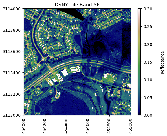
plot_aop_refl: plot a single band of the reflectance data

Next we'll use the function plot_aop_refl to plot a single band of reflectance data. You can use help to understand the required inputs and data types for each of these; only the band and spatial extent are required inputs, the rest are optional inputs. If specified, these optional inputs allow you to set the range color values, specify the axis, add a title, colorbar, colorbar title, and change the colormap (default is to plot in greyscale).

band56 = refl[:,:,55]

neon_hs.plot_aop_refl(band56/refl_metadata['scale_factor'],
                      refl_metadata['extent'],
                      colorlimit=(0,0.3),
                      title='DSNY Tile Band 56',
                      cmap_title='Reflectance',
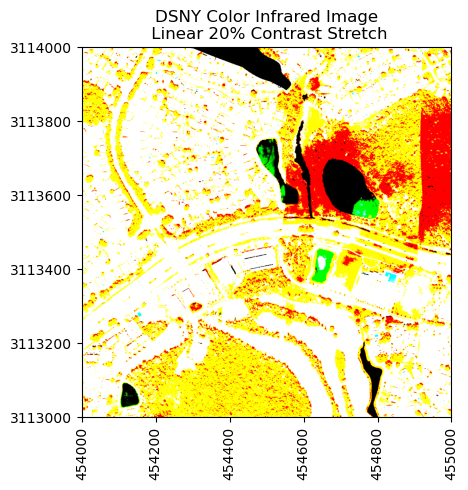
                      colormap='gist_earth')

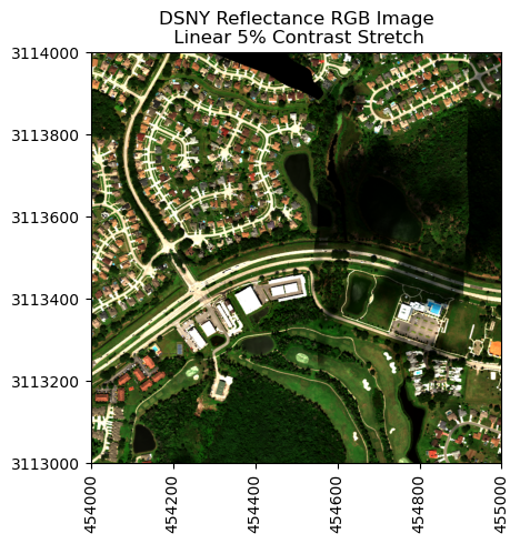
RGB Plots - Band Stacking

It is often useful to look at several bands together. We can extract and stack three reflectance bands in the red, green, and blue (RGB) spectrums to produce a color image that looks like what we see with our eyes; this is your typical camera image. In the next part of this tutorial, we will learn to stack multiple bands and make a geotif raster from the compilation of these bands. We can see that different combinations of bands allow for different visualizations of the remotely-sensed objects and also conveys useful information about the chemical makeup of the Earth's surface.

We will select bands that fall within the visible range of the electromagnetic spectrum (400-700 nm) and at specific points that correspond to what we see as red, green, and blue.

For this exercise, we'll first use the function stack_rgb to extract the bands we want to stack. This function uses splicing to extract the nth band from the reflectance array, and then uses the numpy function stack to create a new 3D array (1000 x 1000 x 3) consisting of only the three bands we want.

# pull out the true-color band combinations
rgb_bands = (58,34,19) # set the red, green, and blue bands

# stack the 3-band combinations (rgb and cir) using stack_rgb function
rgb_unscaled = neon_hs.stack_rgb(refl,rgb_bands)

# apply the reflectance scale factor
rgb = rgb_unscaled/refl_metadata['scale_factor']

We can display the red, green, and blue band center wavelengths, whose indices were defined above. To confirm that these band indices correspond to wavelengths in the expected portion of the spectrum, we can print out the wavelength values in nanometers.

print('Center wavelengths:')
print('Band 58: %.1f' %(wavelengths[57]),'nm')
print('Band 33: %.1f' %(wavelengths[33]),'nm')
print('Band 19: %.1f' %(wavelengths[18]),'nm')

Center wavelengths:
Band 58: 669.3 nm
Band 33: 549.1 nm
Band 19: 474.0 nm

plot_aop_rgb: plot an RGB band combination

Next, we can use the function plot_aop_rgb to plot the band stack as follows:

# plot the true color image (rgb)
neon_hs.plot_aop_rgb(rgb,
                     refl_metadata['extent'],
                     plot_title='DSNY Reflectance RGB Image')

False Color Image - Color Infrared (CIR)

We can also create an image from bands outside of the visible spectrum. An image containing one or more bands outside of the visible range is called a false-color image. Here we'll use the green and blue bands as before, but we replace the red band with a near-infrared (NIR) band.

For more information about non-visible wavelengths, false color images, and some frequently used false-color band combinations, refer to NASA's Earth Observatory page.

cir_bands = (90,34,19)
print('Band 90 Center Wavelength = %.1f' %(wavelengths[89]),'nm')
print('Band 34 Center Wavelength = %.1f' %(wavelengths[33]),'nm')
print('Band 19 Center Wavelength = %.1f' %(wavelengths[18]),'nm')

cir = neon_hs.stack_rgb(refl,cir_bands)
neon_hs.plot_aop_rgb(cir,
                     refl_metadata['extent'],
                     ls_pct=20,
                     plot_title='DSNY Color Infrared Image')

Clipping input data to the valid range for imshow with RGB data ([0..1] for floats or [0..255] for integers).


Band 90 Center Wavelength = 829.6 nm
Band 34 Center Wavelength = 549.1 nm
Band 19 Center Wavelength = 474.0 nm

References

Kekesi, Alex et al. "NASA | Peeling Back Landsat's Layers of Data". https://svs.gsfc.nasa.gov/vis/a010000/a011400/a011491/. Published on Feb 24, 2014.

Riebeek, Holli. "Why is that Forest Red and that Cloud Blue? How to Interpret a False-Color Satellite Image" https://earthobservatory.nasa.gov/Features/FalseColor/

In this tutorial you will learn how to open a .tiff file in Jupyter Notebook and learn about kernels.

The goal of the activity is simply to ensure that you have basic familiarity with Jupyter Notebooks and that the environment, especially the gdal package is correctly set up before you pursue more programming tutorials. If you already are familiar with Jupyter Notebooks using Python, you may be able to complete the assignment without working through the instructions.

Assignment: Open a Tiff File in Jupyter Notebook

Set up Environment

First, we will set up the environment as you would need for each of the live coding sections of the Data Institute. The following directions are copied over from the Data Institute Set up Materials.

In your terminal application, navigate to the directory (cd) that where you want the Jupyter Notebooks to be saved (or where they already exist).

We need to create a new Jupyter kernel for the Python 3.8 conda environment (py38) that Jupyter Notebooks will use.

In your Command Prompt/Terminal, type:

python -m ipykernel install --user --name py34 --display-name "Python 3.8 NEON-RSDI"

In your Command Prompt/Terminal, navigate to the directory (cd) that you created last week in the GitHub materials. This is where the Jupyter Notebook will be saved and the easiest way to access existing notebooks.

###Open Jupyter Notebook Open Jupyter Notebook by typing into a command terminal:

jupyter notebook

Once the notebook is open, check which version of Python you are in.

 # Check what version of Python.  Should be 3.8. 
 import sys
 sys.version

To ensure that the correct kernel will operate, navigate to Kernel in the menu, select Kernel/Restart Kernel And Clear All Outputs.

You should now be able to work in the notebook.

#Download the digital terrain model (GEOTIFF file) Download the NEON GeoTiFF file of a digital terrain model (dtm) of the San Joaquin Experimental Range. Click this link to download dtm data: https://ndownloader.figshare.com/articles/2009586/versions/10. This will download a zippped full of data originally from a NEON data carpentry tutorial (https://datacarpentry.org/geospatial-workshop/data/).

Once downloaded, navigate through the folder to C:NEON-DS-Airborne-Remote-Sensing.zip\NEON-DS-Airborne-Remote-Sensing\SJER\DTM and save this file onto your own personal working directory. .

###Open GEOTIFF file in Jupyter Notebooks using gdal

The gdal package that occasionally has problems with some versions of Python. Therefore test out loading it using:

import gdal.

If you have trouble, ensure that 'gdal' is installed on your current environment.

Establish your directory

Place the downloaded dtm file in a repository of your choice (or your current working directory). Navigate to that directory. wd= '/your-file-path-here' #Input the directory to where you saved the .tif file

Import the TIFF

Import the NEON GeoTiFF file of the digital terrain model (DTM) from San Joaquin Experimental Range. Open the file using the gdal.Open command.Determine the size of the raster and (optional) plot the raster.

#Use GDAL to open GEOTIFF file stored in your directory SJER_DTM = gdal.Open(wd + 'SJER_dtmCrop.tif')>

#Determine the raster size.

  SJER_DTM.RasterXSize

Add in both code chunks and text (markdown) chunks to fully explain what is done. If you would like to also plot the file, feel free to do so.

Push .ipynb to GitHub.

When finished, save as a .ipynb file.